Practice 3: Global navigation
- Final version:
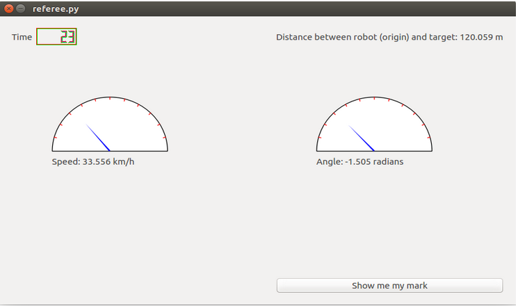
- Referee:
- Examples of final version:
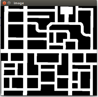
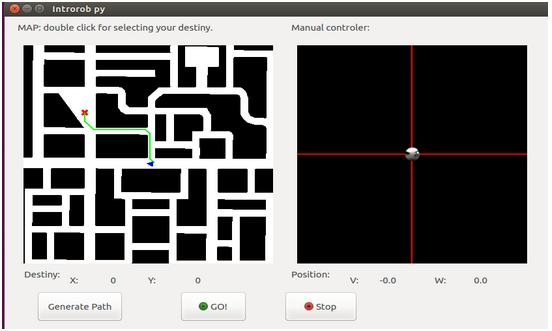
In this practice the objective is to implement the logic of GPP algorithm (Gradient Path Planning). The objective is to reach a marked destination on a map, for this purpose we will use global navigation using the algorithm GPP. We have t choose a destination on the grid. Once marked the destiny, it will expand an imaginary field from the destination until it reaches a bit beyond the robot, to leave a margin in the calculation of the field. The value of this field will increase with the distance to the destination. We will also have to know that there are points that are road and points that are obstacle, for this we have a map image of the city where you have to move the car, (which can be obtained with the grid.getMap() function) where the pixels with value 255 are road and pixels with value 0 are obstacles. The map image provided we can see it below:
To make this practice we will use the platform JdeRobot (we base on the code), the Gazebo simulator, the OpenCV library and as Python programming language. To evaluate the field we divide the process into two parts: the expansion of the field, regardless of penalties for obstacles; and penalties for obstacles.
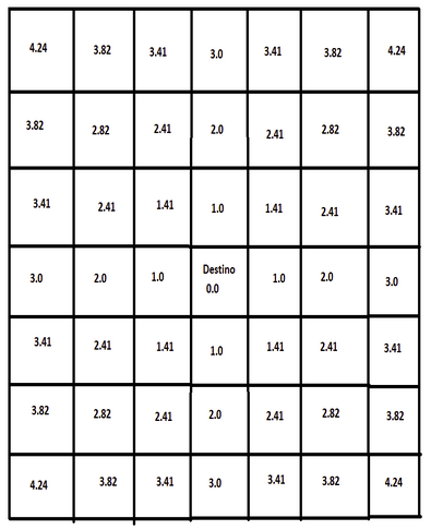
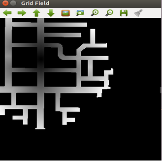
We’ll start first with the expansion of the field. To do this we will put a very high value on the pixels that are obstacle for the cells to be unelected obstacle when we calculate the shortest path.The field will expand as a wavefront if it were, the first wavefront will start at the destination. To propagate the wavefront, we must bear in mind that we have a grid where we will be writing down the values with the grid.setVal(x, y, val) function. When performing expansion, we must consider whether the destination is road or obstacle. If the destination is a way we can put the value 0 and if is obstacle will put a very high value, for example 20000. To calculate the value of neighboring cells, we must keep in mind that in the first iteration the destination will put the value to its 8 neighbors. In the cells that are diagonally with respect to the destination, we will put a value equal to the value of the destination cell √2, and in the rest we will put a value equal to the value of the destination cell plus 1. In the next iteration, the 8 neighbors of the destination will also want to spread, so for each of these 8 neighbors will assess the value of its 8 neighbors concerned. To do this, we will have to see if the cell had a value, if so, we decide to put the smallest value. In addition we follow the same logic as in the case of destination, if we are in cells that are located on the diagonal, we increase the field in √2, and if they are adjacent to another position will increase by 1 the value of the central pixel. If the pixel that we are evaluating has a value nan, a negative value or the value is zero (but the cell does not match the destination), then we have to put a value on that cell, as this means that no previous pixel had spread its field to this cell. If we look to the expansion of the third wavefront and that all cells are part of the way, the field values would be as follows:
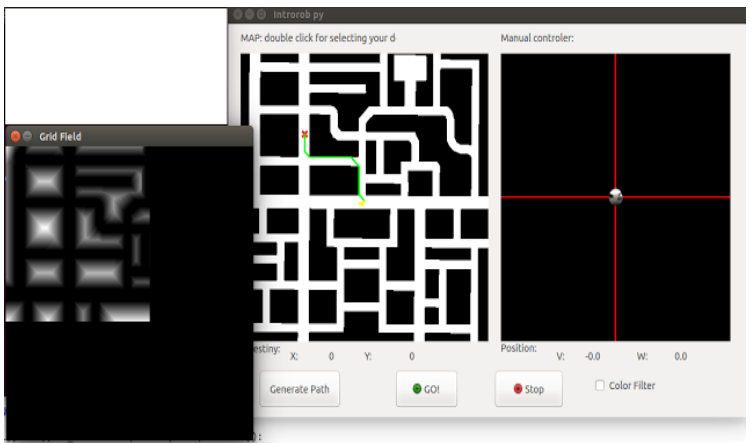
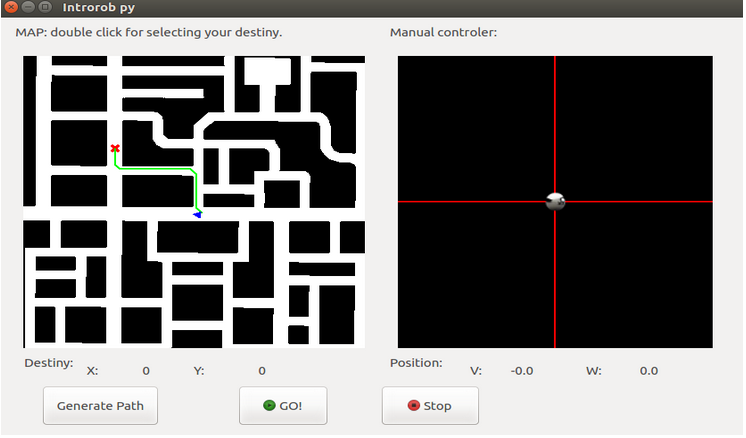
After we should add a penalty to the pixels of the road that are very close to obstacles. We must also find the shortest path from the robot to the destination. What we do is look at the 8 neighbors of the robot and we will keep the neighbor who has a smaller value in the grid. Then we look at the 8 neighbors of this pixel, and thus continuously to reach the destination. So we’ll build the shortest path from the robot to the destination. To do this we use the grid.setPathVal function (x, y, val), which sets the value val at the position indicated, and also use the grid.setPathFinded () function, which states that it has already found the way and it can be painted. Here we can see an image of the shortest path without the penalties of obstacles:
Here we can see a video of the field’s expansion:
Then we have to make the penalty for obstacles.We will have to increase the value of the pixels that are very close to the obstacles. f the pixel is next to an obstacle we put penalty 25. If the pixel is next to the previous pixel we put penalty 15. If the pixel is next to the previous pixel we put penalty 10.Here we can see an image of the shortest path with the penalties of obstacles:
Here we can see a video of the obstacles’ penalties:
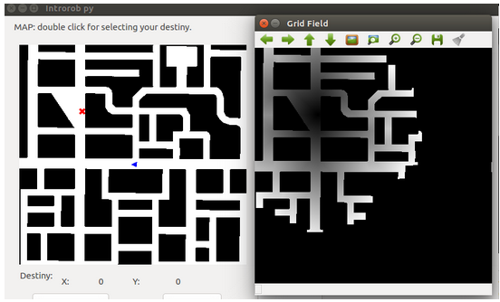
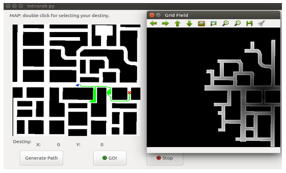
I’ve done some changes. The new field’s expansion is:
And the obstacles’ penalties:

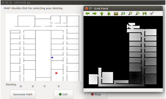
I’ve done more testing with other maps:
I’ve calculated the shortest route:
I had some problems calculating the route, because sometimes local minimum are generated. I’ve solved it. I’ve done tests:

New video:
More test:
New taxi:
Test with changes: