Datasets - Data types
We will handle data of different nature that increase the degree of difficulty. The code to generate these samples can be found here
Linear Functions dataset
It is the simplest data to handle. The input of the network is a sequence of 20 numbers that follow the function of a line (y = m/t + n) and the value that the network will return to us is the corresponding value of the function at point 20 + gap. The samples are stored in a *.txt file in which each line corresponds to a sample and the values of the function are stored in points [0,19] and 19 + gap. In the following figure you can see an example of a sample of this type of functions:
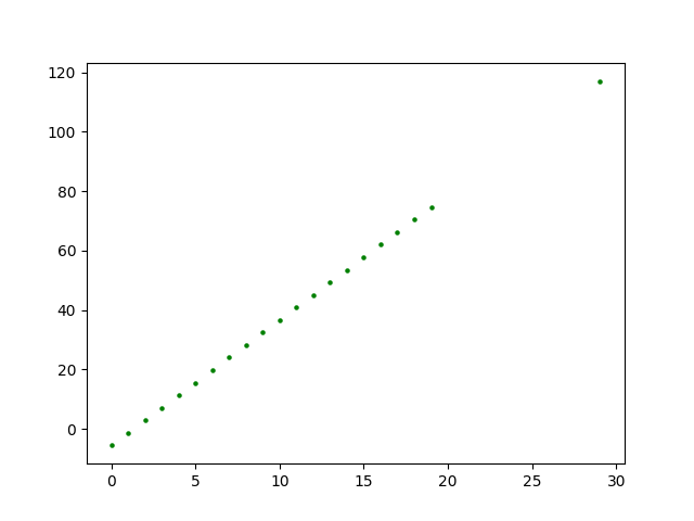
To reduce complexity and avoid infinite slope lines, samples have been generated with a limitation in their slope defined in the configuration file.
URM Vectors dataset
We increase the complexity of the previous data by increasing a dimension. We have created several 1D images in which the position of an object is represented at each moment of time. Each sample consists of 20 + 1 vectors, so that each vector consists of 320 positions and only activates (has a value of 255) that corresponds to the position in which the object would be found. To calculate the position we use a URM movement formula.
  f = lambda t: x0 + u_x * t
  u_x = random.randint(1, int(self.v_size[1] / (n_points + gap)))
  x0 = 0
In the following figure you can see an example of a sample of this type of samples:

The 2D image represents in each row a continuous moment of time with the exception of the last row that corresponds to the position to be predicted with a gap of 10. In addition, the speed of the object is limited so that in the prediction the object is always in the image.
Frames dataset
The next step to increase the complexity is to increase one more dimension. In this way, each sample will consist of 20 + 1 images (frames) in which the movement of an object will be represented through the time with a single pixel.
URM Point
The first and easiest step is to modify only the horizontal pixel position (x) using the URM formula, leaving the height (y) constant.
  f = lambda t, x0, u_x: x0 + u_x * t
  g = lambda x, y0: y0
In the following video you can see an example of a sample of this type of samples:
As in the previous case, the speed of the object is limited so that in the prediction the object is always in the image.
Linear motion
We add a new degree of complexity by modifying the pixel height in the image (y) by linear motion, as for the position x we will keep the URM movement.
  f = lambda t, x0, u_x: x0 + u_x * t
  g = lambda x, y0, m: (m * x) + y0
In this first case we keep the initial height (y0) constant in the middle of the image and modify the m value:
  m = np.round(random.uniform(-self.h/10, self.h/10), 2)
  y0 = int(height/2)
And in the next you can see a sample of this:
Random initial height
The equations that govern this new data type are the same as in the previous case, but now we will give the position y0 a random value within the range of the frame:
y0 = y0 = random.randint(0, height - 1)
With this new degree of freedom we increase the variety in the samples and complicate the problem to the neural network to predict the desired value. Below you can see an example of these new samples:
Parabolic motion
In this case we modify the motion type that is applied to calculate the height (y) of the pixel, using a parabolic function, while the way to calculate the x position continues to be the URM motion.
  f = lambda t, x0, u_x: x0 + u_x * t
  g = lambda x, a, b, c: a * (x ** 2) + b * x + c
In a first approximation we will keep two of the variables of the equation (b and c) constant and we will only modify the value of a in each sample.
  a = round(random.uniform(-0.75, 0.75), 3)
  b = 1.5
  c = y0 = int(self.h / 2)
Below you can see an example of these new samples:
Sinusoidal motion
In this new data type we keep the x position governed by the URM movement again and we will modify the value of y with a sinusoidal equation.
  f = lambda t, x0, u_x: x0 + u_x * t
  g = lambda x, a, b, c, f: a * math.sin(2 * math.pi * f * math.radians(x) + b) + c
As in the case of the parabolic we start by keeping all the values constant except for the frequency (f).
  a = 25
  b = math.radians(0)
  c = y0 = int(self.h / 2)
  f = round(random.uniform(0.5, 5), 2)
Below you can see an example of these new samples: