Week 11: Correction of the binary classification model, correction of driver node, accuracy top2, Pilotnet network

Correction of the binary classification model

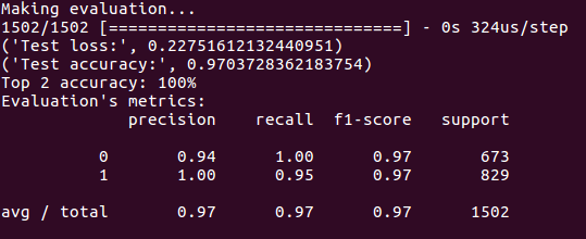
I modified the binary classification models/model_classification.h5, which had some error. That model has been removed and is now called model_binary_classification.h5. After training the network, we save the model (models/model_binary_classification.h5) and evaluate the model with the validation set:

In addition, we evaluate the accuracy, precision, recall, F1-score and we paint the confusion matrix. The results are the following:

Correction of driver node

The driver node had an error that caused Formula 1 to stop sometimes. This error was due to the fact that the telemarketer was interfering with the speed of the vehicle. This error has been corrected and the F1 can be driven correctly.

Accuracy top 2 of multiclass classification network

To get an idea of ​​the results with the multiclass classification network that we trained previously, we have obtained a measure of accuracy top 2. To obtain this metric we give as good a prediction if it is equal to the true label or if it is equal to the adjacent label, that is, we take into account only 1 accuracy jump. In this way we obtain a 100% accuracy.

Pilotnet network

This week, one of the objectives was to train a regression network to learn values ​​of linear speed and angular speed of the car. For this we’ve followed the article Explaining How to Deep Neural Network Trained with End-to-End Learning Steers to Car and we’ve created a network with the Pilotnet architecture. NVIDIA has created a neural-network-based system, known as PilotNet, which outputs steering angles given images of the road ahead. PilotNet is trained using road images paired with the steering angles generated by a human driving a data-collection car. In our case we have pairs of images and (v, w). The Pilonet architecture is as follows:

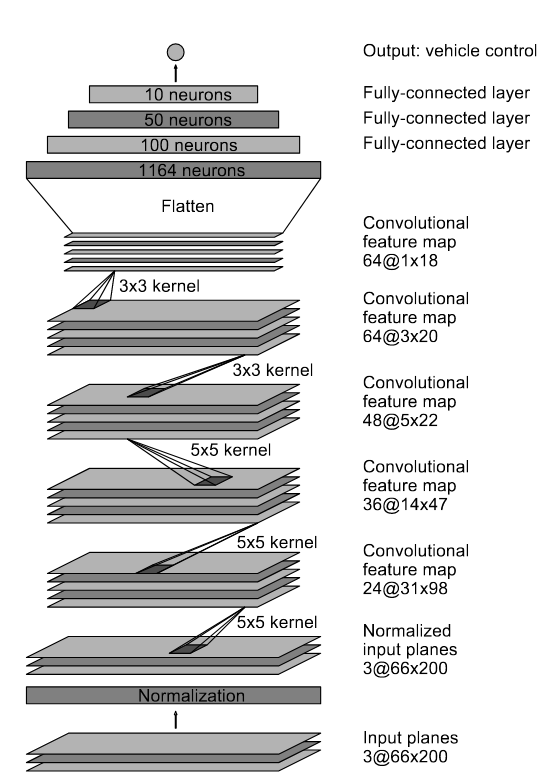
The Pilotnet model can be seen below:

model = Sequential()
# Normalization
model.add(BatchNormalization(epsilon=0.001, axis=-1, input_shape=img_shape))
# Convolutional layer
model.add(Conv2D(24, (5, 5), strides=(2, 2), activation="relu", input_shape=img_shape))
# Convolutional layer
model.add(Conv2D(36, (5, 5), strides=(2, 2), activation="relu"))
# Convolutional layer
model.add(Conv2D(48, (5, 5), strides=(2, 2), activation="relu"))
# Convolutional layer
model.add(Conv2D(64, (3, 3), strides=(1, 1), activation="relu"))
# Convolutional layer
model.add(Conv2D(64, (3, 3), strides=(1, 1), activation="relu"))
# Flatten
model.add(Flatten())
model.add(Dense(1164, activation="relu"))
# Fully-connected layer
model.add(Dense(100, activation="relu"))
# Fully-connected layer
model.add(Dense(50, activation="relu"))
# Fully-connected layer
model.add(Dense(10, activation="relu"))
# Output: vehicle control
model.add(Dense(1))
model.compile(optimizer="adam", loss="mse", metrics=['accuracy'])

In order to learn the angular speed (w) and the linear speed (v) we train two networks, one for each value. The model for v is called model_pilotnet_v.h5 and the model for w is called model_pilotnet_w.h5.

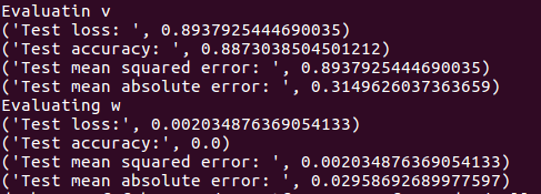
After training the networks, we save the models (models/model_pilotnet_v.h5, models/model_pilotnet_w.h5) and evaluate (loss, accuracy, mean squared error and mean absolute error) the models with the validation set:

In addition, we evaluate the networks with the test set:

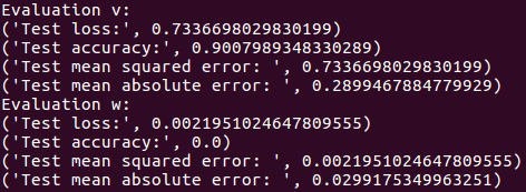
The w’s evaluation had a problem. This problem is fixed and the result is:

Evaluation w:
('Test loss:', 0.0021951024647809555)
('Test accuracy:', 0.0)
('Test mean squared error: ', 0.0021951024647809555)
('Test mean absolute error: ', 0.0299175349963251)