Week 13: Data’s Analysis, New Dataset

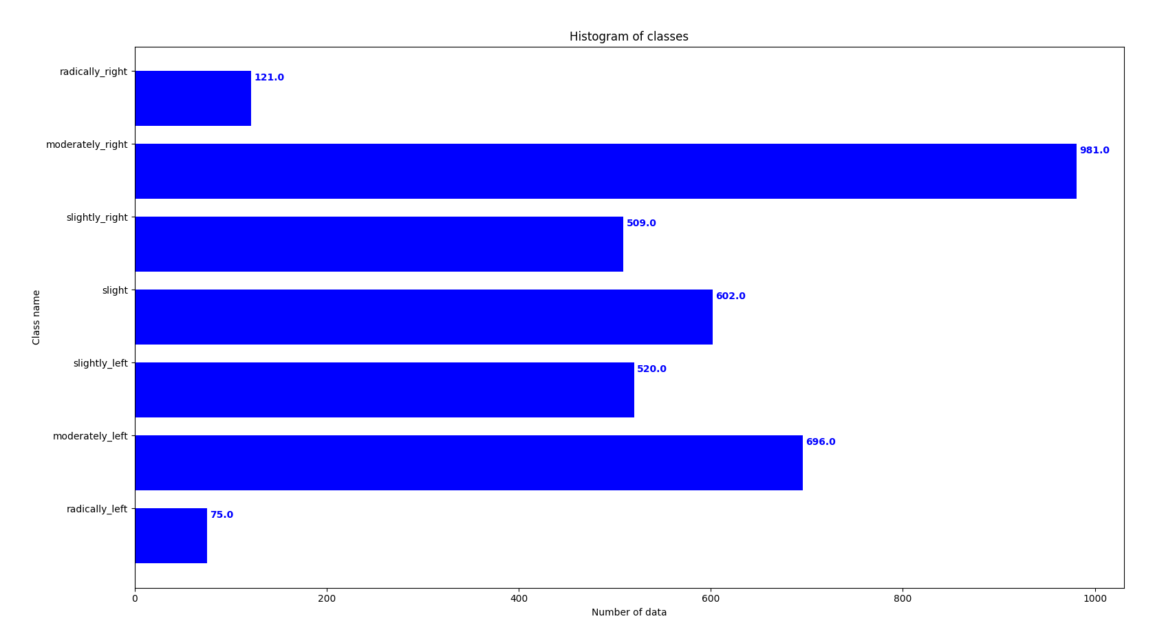
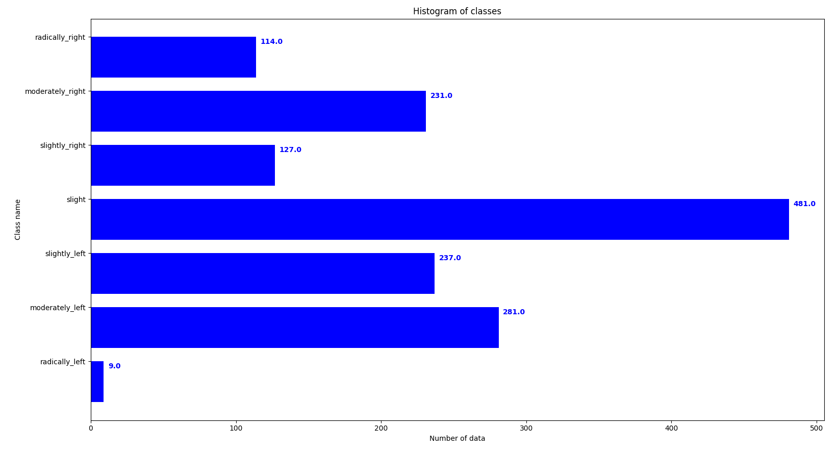
Number of data for each class

At 1 we saw that the car was not able to complete the entire circuit with the classification network of 7 classes and constant v. For this reason, we want to evaluate our dataset and see if it is representative. For this we’ve saved the images that the F1 sees during the driving with the neural network and some data. This data can be found at Github.

I’ve created a script (evaluate_class.py) that shows a graph of the number of examples that exist for each class (7 classes of w). In the following images we can see first the graph for the training data and then the graph for the driving data.

Data statistics

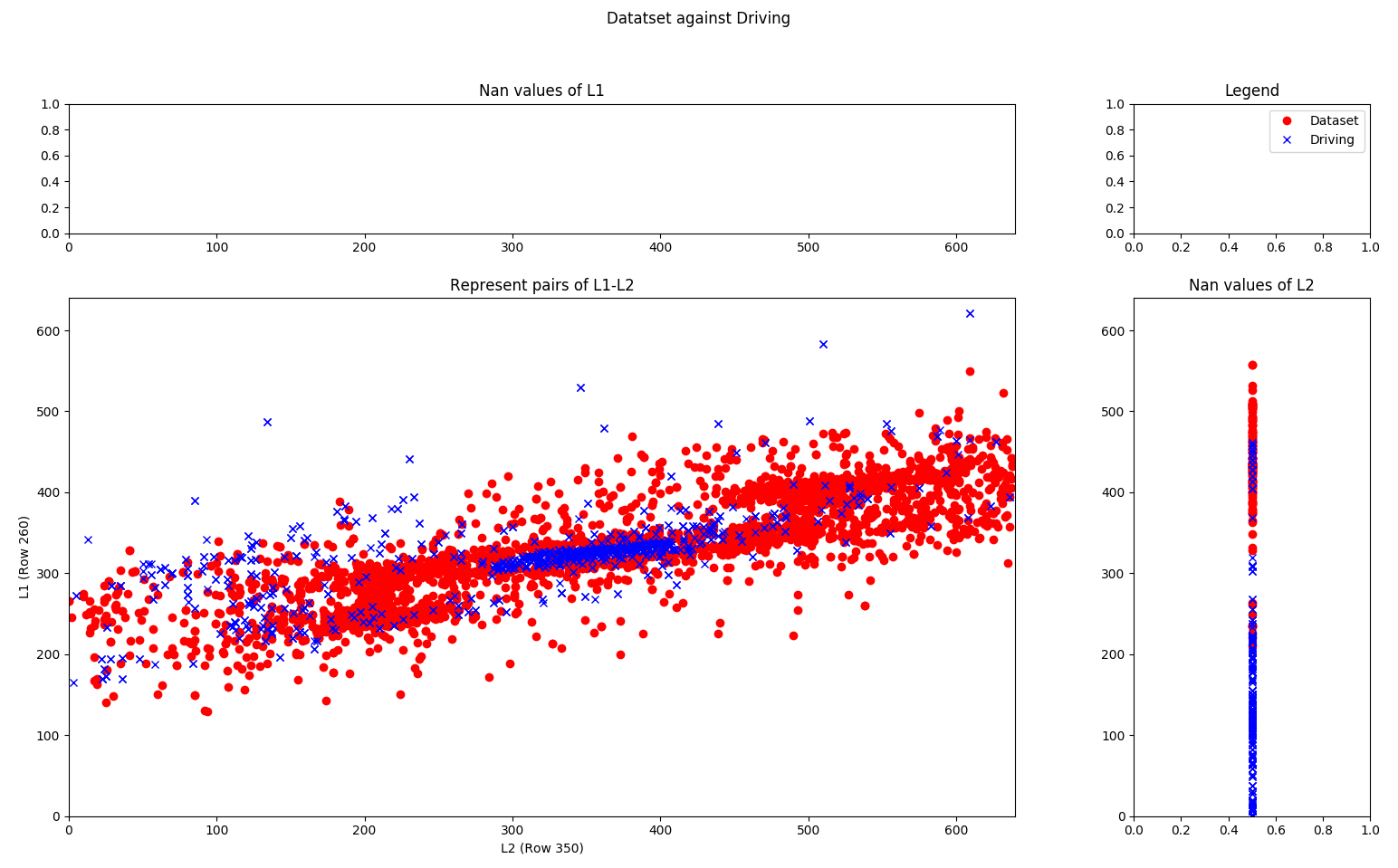
To analyze the data, a new statistic was created (analysis_vectors.py). I’ve analyzed two lines of each image and calculated the centroids of the corresponding lines (row 250 and row 360). On the x-axis of the graph, the centroid of row 350 is represented and the y-axis represents the centroid of row 260 of the image. In the following image we can see the representation of this statistic of the training set (red circles) iagainst the driving data (blue crosses).

Entropy

I’ve used the entropy how measure of simility. The Shannon entropy is the measure of information of a set. Entropy is defined as the expected value of the information. I’ve follow a Python example of the book Machine Learning In Action. In this book uses the following function to calculate the Shannon entropy of a dataset:

def calculate_shannon_entropy(dataset):
    numEntries = len(dataset)
    labelCounts = {}
    for featVec in dataset: #the the number of unique elements and their occurance
        currentLabel = featVec[-1]
        if currentLabel not in labelCounts.keys(): labelCounts[currentLabel] = 0 
        labelCounts[currentLabel] += 1
    print(labelCounts)
    shannonEnt = 0.0
    for key in labelCounts:
        prob = float(labelCounts[key])/numEntries
        shannonEnt -= prob * log(prob,2) #log base 2
    return shannonEnt

First, you calculate a count of the number of instances in the dataset. This could have been calculated inline, but it’s used multiple times in the code, so an explicit variable is created for it. Next, you create a dictionary whose keys are the values in the final column. If a key was not encountered previously, one is created. For each key, you keep track of how many times this label occurs. Finally, you use the frequency of all the different labels to calculate the probability of that label. This probability is used to calculate the Shannon entropy, and you sum this up for all the labels.

In this example the dataset is:

[[1, 1, 'yes'], [1, 1, 'yes'], [1, 0, 'no'], [0, 1, 'no'], [0, 1, 'no']]

In my case, we want to measure the entropy of train set and entropy of driving train. In my case, I haven’t used the labels and I’ve used the centroid of 3 rows of images. For this reason, I’ve modified the function “calculate_shannon_entropy”:

def calculate_shannon_entropy(dataset):
    numEntries = len(dataset)
    labels = []
    counts = []
    for featVec in dataset: #the the number of unique elements and their occurance
        found = False
        for i in range(0, len(labels)):
            if featVec == labels[i]:
                found = True
                counts[i] += 1
        if not found:
            labels.append(featVec)
            counts.append(0)
    shannonEnt = 0.0
    for num in counts:
        prob = float(num)/numEntries
        shannonEnt -= prob * log(prob,2) #log base 2
    return shannonEnt

My dataset is like:

[[32, 445, 34], [43, 12, 545], [89, 67, 234]]

The entropy’s results are:

Shannon entropy of driving: 0.00711579828413
Shannon entropy of dataset: 0.00336038443482

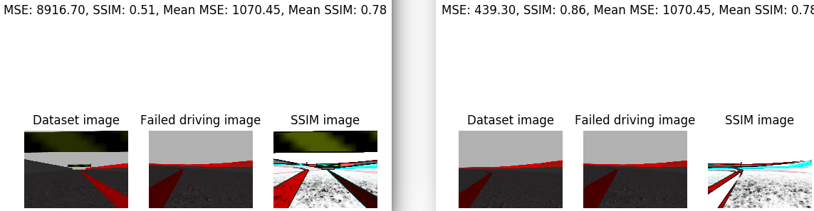
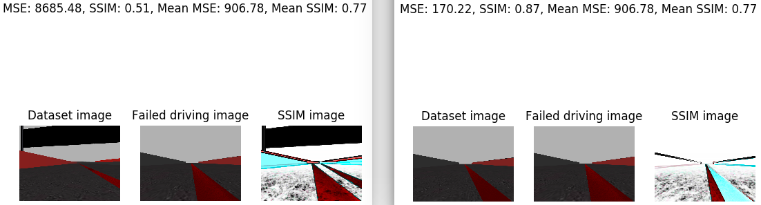
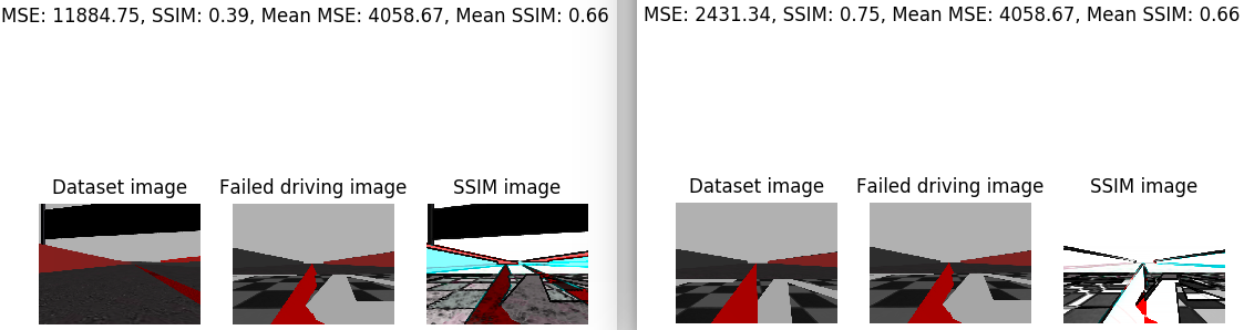
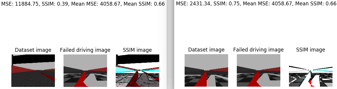
SSIM and MSE

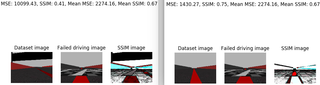
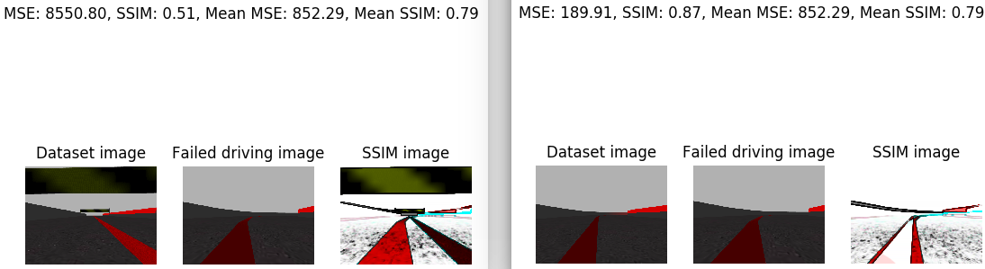
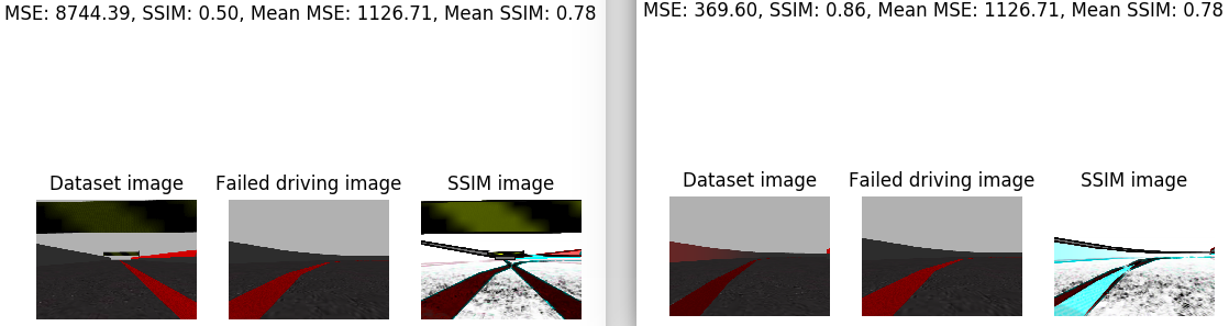
In addition, to verify the difference between the piloting data and the training data I’ve used the SSIM and MSE measurements. The MSE value is obtained, although it isn’t a very representative value of the similarity between images. Structural similarity aims to address this shortcoming by taking texture into account.

The Structural Similarity (SSIM) index is a method for measuring the similarity between two images. The SSIM index can be viewed as a quality measure of one of the images being compared, provided the other image is regarded as of perfect quality.

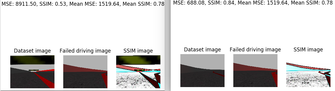
I’ve analyzed the image that the car saw just before leaving the road. I’ve compared this image with the whole training set. For this I’ve calculated the average SSIM. In addition, I’e calculated the minimum SSIM and the maximum SSIM. The minimum SSIM is given in the case that we compare our image with a very disparate one. And the maximum SSIM is given in the case that we compare the image with the one that is closest to the training set. Next, the case of the minimum SSIM is shown on the left side and the case of the maximum SSIM on the right side. For each case, the corresponding SSIM, the MSE, the medium SSIM, the average MSE, the image, the iamgen of the dataset with which the supplied SSIM corresponds, and the SSIM image are printed.

In addition, the same images are provided for a piloting image of each class of w.

• ‘radically_left’:

• ‘moderately_left’:

• ‘slightly_left’:

• ‘slight’:

• ‘slightly_right’:

• ‘moderately_right’:

• ‘radically_right’:

New Dataset

I’ve based on the code created for the follow-line practice of JdeRobot Academy in order to create a new dataset. This new dataset has been generated using 3 circuits so that the data is more varied. The circuits of the worlds monacoLine.world, f1.launch and f1-chrono.launch have been used.