Week 20: Driving videos, Reading information

Driving videos

Biased classfication network

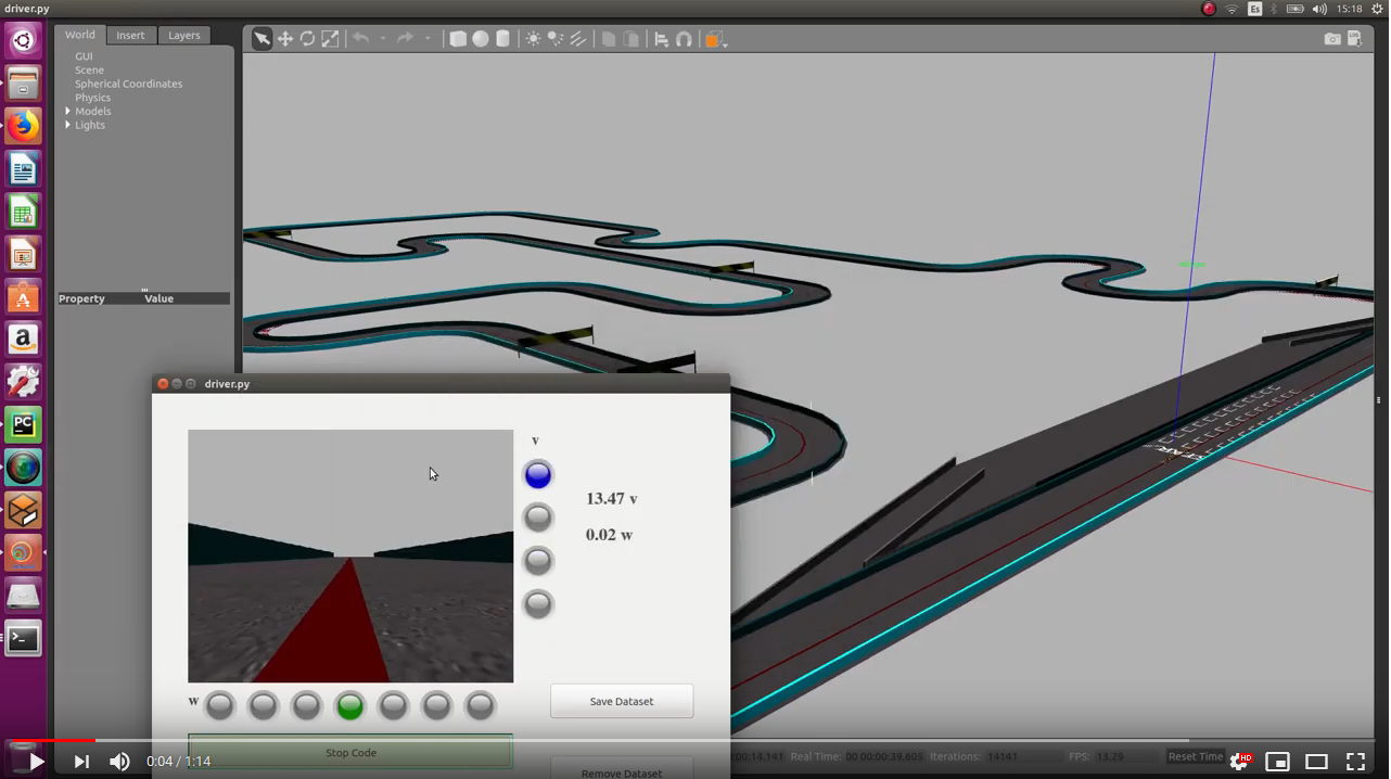
I’ve used the predictions of the classification network according to w (7 classes) and constant v to driving a formula 1 (simulation time: 2min 17s):

Balanced classfication network

I’ve used the predictions of the classification network according to w (7 classes) and constant v to driving a formula 1:

Pilotnet network

I’ve used the predictions of the pilotnet network (regression network) to driving a formula 1 (test1):

I’ve used the predictions of the pilotnet network (regression network) to driving a formula 1 (test2):

I’ve used the predictions of the pilotnet network (regression network) for w and constant v to driving a formula 1 (simulation time: 3min 46s):

Reading information

This week, I read some papers about Deep Learning for Steering Autonomous Vehicles. Some of these papers are:

Interpretable Learning for Self-Driving Cars by Visualizing Causal Attention

In this paper, they use a visual attention model to train a convolution network end-to-end from images to steering angle. The attention model highlights image regions that potentially influence the network’s output. Some of these are true influences, but some are spurious. They then apply a causal filtering step to determine which input regions actually influence the output. This produces more succinct visual explanations and more accurately exposes the network’s behavior. They demonstrate the effectiveness of their model on three datasets totaling 16 hours of driving. they first show that training with attention does not degrade the performance of the end-to-end network. Then they show that the network causally cues on a variety of features that are used by humans while driving.

Their model predicts continuous steering angle commands from input raw pixels in an end-to-end manner. Their model predicts the inverse turning radius ût at every timestep t instead of steering angle commands, which depends on the vehicle’s steering geometry and also result in numerical instability when predicting near zero steering angle commands. The relationship between the inverse turning radius ut and the steering angle command θt can be approximated by Ackermann steering geometry.

To reduce computational cost, each raw input image is down-sampled and resized to 80×160×3 with nearest-neighbor scaling algorithm. For images with different raw aspect ratios, they cropped the height to match the ratio before down-sampling. They also normalized pixel values to [0, 1] in HSV colorspace. They utilize a single exponential smoothing method to reduce the effect of human factors-related performance variation and the effect of measurement noise.

They use a convolutional neural network to extract a set of encoded visual feature vector, which we refer to as a convolutional feature cube xt. Each feature vectors may contain high-level object descriptions that allow the attention model to selectively pay attention to certain parts of an input image by choosing a subset of feature vectors. They use a 5-layered convolution network that is utilized by Bojarski (https://arxiv.org/pdf/1604.07316.pdf) to learn a model for self-driving cars. They omit max-pooling layers to prevent spatial locational information loss as the strongest activation propagates through the model. They collect a three-dimensional convolutional feature cube xt from the last layer by pushing the preprocessed image through the model, and the output feature cube will be used as an input of the LSTM layers. Using this convolutional feature cube from the last layer has advantages in generating high-level object descriptions, thus increasing interpretability and reducing computational burdens for a real-time system.

They utilize a deterministic soft attention mechanism that is trainable by standard backropagation methods, which thus has advantages over a hard stochastic attention mechanism that requires reinforcement learning. They use a long short-term memory (LSTM) network that predicts the inverse turning radius and generates attention weights each timestep t conditioned on the previous hidden state and a current convolutional feature cube xt. More formally, let us assume a hidden layer conditioned on the previous hidden state and the current feature vectors. The attention weight for each spatial location i is then computed by multinomial logistic regression function.

The last step of their pipeline is a fine-grained decoder, in which they refine a map of attention and detect local visual saliencies. Though an attention map from their coarse-grained decoder provides probability of importance over a 2D image space, their model needs to determine specific regions that cause a causal effect on prediction performance. To this end, they assess a decrease in performance when a local visual saliency on an input raw image is masked out. They first collect a consecutive set of attention weights and input raw images for a user-specified T timesteps. They then create a map of attention (Mt). Their 5-layer convolutional neural network uses a stack of 5×5 and 3×3 filters without any pooling layer, and therefore the input image of size 80×160 is processed to produce the output feature cube of size 10×20×64, while preserving its aspect ratio. To extract a local visual saliency, they first randomly sample 2D N particles with replacement over an input raw image conditioned on the attention map Mt. They also use time-axis as the third dimension to consider temporal features of visual saliencies. They thus store spatio-temporal 3D particles. They then apply a clustering algorithm to find a local visual saliency by grouping 3D particles into clusters. In their experiment, they use DBSCAN, a density-based clustering algorithm that has advantages to deal with a noisy dataset because they group particles together that are closely packed, while marking particles as outliers that lie alone in low-density regions. For points of each cluster and each time frame t, they compute a convex hull to find a local region of each visual saliency detected.

Event-based Vision meets Deep Learning on Steering Prediction for Self-driving Cars

This paper, (2) presents a deep neural network approach that unlocks the potential of event cameras on the prediction of a vehicle’s steering angle. They evaluate the performance of their approach on a publicly available large scale event-camera dataset (≈1000 km). They present qualitative and quantitative explanations of why event cameras (bio-inspired sensors that do not acquire full images at a fixed frame-rate but rather have independent pixels that output only intensity changes asynchronously at the time they occur) allow robust steering prediction even in cases where traditional cameras fail. Finally, they demonstrate the advantages of leveraging transfer learning from traditional to event-based vision, and show that their approach outperforms state-of-the-art algorithms based on standard cameras.

They propose a learning approach that takes as input the visual information acquired by an event camera and outputs the vehicle’s steering angle. The events are converted into event frames by pixel-wise accumulation over a constant time interval. Then, a deep neural network maps the event frames to steering angles by solving a regression task.

They preprocess the data. The steering angle’s distribution of a driving car is mainly picked in [−5º, 5º]. This unbalanced distribution results in a biased regression. In those situations where vehicles stand still, only noisy events will be produced. To handle those problems, they preprocessed the steering angles to allow successful learning. To cope with the first issue, only 30 % of the data corresponding to a steering angle lower than 5º is deployed at training time. For the latter they filtered out data corresponding to a vehicle’s speed smaller than 20km/h. To remove outliers, the filtered steering angles are then trimmed at three times their standard deviation and normalized to the range [−1, 1]. At testing time, all data corresponding to a steering angle lower than 5º is considered, as well as scenarios under 20km/h. The regressed steering angles are denormalized to output values in the range [−180º, 180º]. Finally, they scaled the network input (i.e., event images) to the range [0, 1].

Initially, they stack event frames of different polarity, creating a 2D event image. Afterwards, they deploy a series of ResNet architectures, i.e., ResNet18 and ResNet50. They use them as feature extractors for their regression problem, considering only their convolutional layers. To encode the image features extracted from the last convolutional layer into a vectorized descriptor, they use a global average pooling layer that returns the features’ channel-wise mean. After the global average pooling, they add a fully-connected (FC) layer (256-dimensional for ResNet18 and 1024-dimensional for ResNet50), followed by a ReLU non-linearity and the final one-dimensional fully-connected layer to output the predicted steering angle.

They use DAVIS Driving Dataset 2017 (DDD17). It contains approximately 12 hours of annotated driving recordings collected by a car under different and challenging weather, road and illumination conditions. It contains approximately 12 hours of annotated driving recordings collected by a car under different and challenging weather, road and illumination conditions. The dataset includes asynchronous events as well as synchronous, grayscale frames.

They predicted steering angles using three different types of visual inputs: 1. grayscale images, 2. difference of grayscale images, 3. images created by event accumulation. To evaluate the performance, they use the root-mean-squared error (RMSE) and the explained variance (EVA).

They analyze the performance of the network as a function of the integration time used to generate the input event images from the event stream (10, 25, 50, 100, and 200 ms). It can be observed that the larger the integration time, the larger is the trace of events appearing at the contours of objects. This is due to the fact that they moved a longer distance on the image plane during that time. They hypothesize that the network exploits such motion cues to provide a reliable steering prediction. The network performs best when it is trained on event images corresponding to 50 ms, and the performance degrades for smaller and larger integration times.

They perform an extensive study to evaluate the advantages of event frames over grayscale-based ones for different parts of the day. For fair comparison, they deploy the same convolutional network architectures as feature encoders for all considered inputs, but we train each network independently. The average RMSE is slightly diverse among different sets. This is to be expected, since RMSE, being dependent on the absolute value of the steering ground truth, is not a good metric for cross comparison between sequences. On the other hand, EVA gives a better way to compare the quality of the learned estimator across different sequences. They we observe a very large performance gap between the grayscale difference and the event images for the ResNet18 architecture. The main reasons behind this behavior that they identified are: (i) abrupt changes in lighting conditions occasionally produced artifacts in grayscale images (and therefore also in their differences), and (ii) at high velocities, grayscale images get blurred and their difference becomes also very noisy. However, that the ResNet50 architecture produced a significant performance improvement for both baselines (grayscale images and difference of grayscale images).

To evaluate the ability of their proposed methodology to cope with large variations in illumination, driving and weather conditions, we trained a single regressor over the entire dataset. They compare their approach to state-of-the-art architectures that use traditional frames as input: (i) Boarski and (ii) the CNN-LSTM architecture, advocated in 3, but without the additional segmentation loss that is not available in their dataset. All their proposed architectures based on event images largely outperform the considered baselines based on traditional frames.