Week 22: Results table, Data analysis, CARLA simulator, Udacity simulator

CARLA simulator

CARLA (1, 2, 3) is an open-source simulator for autonomous driving research. CARLA has been developed from the ground up to support development, training, and validation of autonomous driving systems. In addition to open-source code and protocols, CARLA provides open digital assets (urban layouts, buildings, vehicles) that were created for this purpose and can be used freely. The simulation platform supports flexible specification of sensor suites and environmental conditions.

CARLA simulates a dynamic world and provides a simple interface between the world and an agent that interacts with the world. To support this functionality, CARLA is designed as a server-client system, where the server runs the simulation and renders the scene. The client API is implemented in Python and is responsible for the interaction between the autonomous agent and the server via sockets. The client sends commands and meta-commands to the server and receives sensor readings in return. Commands control the vehicle and include steering, accelerating, and braking. Meta-commands control the behavior of the server and are used for resetting the simulation, changing the properties of the environment, and modifying the sensor suite. Environmental properties include weather conditions, illumination, and density of cars and pedestrians. When the server is reset, the agent is re-initialized at a new location specified by the client.

CARLA allows for flexible configuration of the agent’s sensor suite. Sensors are limited to RGB cameras and to pseudo-sensors that provide ground-truth depth and semantic segmentation. The number of cameras and their type and position can be specified by the client. Camera parameters include 3D location, 3D orientation with respect to the car’s coordinate system, field of view, and depth of field. Its semantic segmentation pseudo-sensor provides 12 semantic classes: road, lane-marking, traffic sign, sidewalk, fence, pole,wall, building, vegetation, vehicle, pedestrian, and other.

CARLA provides a range of measurements associ-ated with the state of the agent and compliance with traffic rules. Measurements of the agent’s stateinclude vehicle location and orientation with respect to the world coordinate system, speed, acceleration vector, and accumulated impact from collisions. Measurements concerning traffic rules include the percentage of the vehicle’s footprint that impinges on wrong-way lanes or sidewalks, as well as states of the traffic lights and the speed limit at the current location ofthe vehicle. Finally, CARLA provides access to exact locations and bounding boxes of all dynamic objects in the environment. These signals play an important role in training and evaluating driving policies.

CARLA has the following features:

Scalability via a server multi-client architecture: multiple clients in the same or in different nodes can control different actors.
Flexible API: CARLA exposes a powerful API that allows users to control all aspects related to the simulation, including traffic generation, pedestrian behaviors, weathers, sensors, and much more.
Autonomous Driving sensor suite: users can configure diverse sensor suites including LIDARs, multiple cameras, depth sensors and GPS among others.
Fast simulation for planning and control: this mode disables rendering to offer a fast execution of traffic simulation and road behaviors for which graphics are not required.
Maps generation: users can easily create their own maps following the OpenDrive standard via tools like RoadRunner.
Traffic scenarios simulation: our engine ScenarioRunner allows users to define and execute different traffic situations based on modular behaviors.
ROS integration: CARLA is provided with integration with ROS via our ROS-bridge.
Autonomous Driving baselines: we provide Autonomous Driving baselines as runnable agents in CARLA, including an AutoWare agent and a Conditional Imitation Learning agent.

CARLA requires Ubuntu 16.04 or later. CARLA consists mainly of two modules, the CARLA Simulator and the CARLA Python API module. The simulator does most of the heavy work, controls the logic, physics, and rendering of all the actors and sensors in the scene; it requires a machine with a dedicated GPU to run. The CARLA Python API is a module that you can import into your Python scripts, it provides an interface for controlling the simulator and retrieving data. With this Python API you can, for instance, control any vehicle in the simulation, attach sensors to it, and read back the data these sensors generate.

Udacity’s Self-Driving Car Simulator

Udacity’s Self-Driving Car Simulator (4) was built for Udacity’s Self-Driving Car Nanodegree, to teach students how to train cars how to navigate road courses using deep learning.

Data analysis

I’ve analyzed the speed data (v and w) of the dataset. In particular, I’ve counted the data number for different speed ranges. For the angular velocity I have divided the angles of 0.3 into 0.3. And I have divided the linear velocities into negative, speed equal to 5, 9, 11 and 13.

The results (number of data) for w are:

w < -2.9             ===> 1
-2.9 <= w < -2.6     ===> 13
-2.6 <= w < -2.3     ===> 20
-2.3 <= w < -2.0     ===> 50
-2.0 <= w < -1.7     ===> 95
-1.7 <= w < -1.4     ===> 165
-1.4 <= w < -1.1     ===> 385
-1.1 <= w < -0.8     ===> 961
-0.8 <= w < -0.5     ===> 2254
-0.5 <= w < -0.2     ===> 1399
-0.2 <= w < -0.0     ===> 3225
0.0 <= w < 0.2       ===> 3399
0.2 <= w < 0.5       ===> 1495
0.5 <= w < 0.8       ===> 2357
0.8 <= w < 1.1       ===> 937
1.1 <= w < 1.4       ===> 300
1.4 <= w < 1.7       ===> 128
1.7 <= w < 2.0       ===> 76
2.0 <= w < 2.3       ===> 41
2.3 <= w < 2.6       ===> 31
2.6 <= w < 2.9       ===> 8
w >= 2.9             ===> 1

The results (number of data) for v are:

v <= 0             ===> 197
v = 5              ===> 9688
v = 9              ===> 3251
v = 11             ===> 2535
v = 13             ===> 1670

Results table (cropped image)

Driving results of classification networks
	Manual	1v+7w biased	4v+7w biased	1v+7w balanced	4v+7w balanced	1v+7w imbalanced	4v+7w imbalanced
Circuits	Percentage	Time	Percentage	Time	Percentage	Time	Percentage	Time	Percentage	Time	Percentage	Time	Percentage	Time
Simple (clockwise)	100%	1min 35s	75%		10%		80%		25%		10%		10%
Simple (anti-clockwise)	100%	1min 32s	25%		15%		65%		65%		100%	2min 16s	25%
Monaco (clockwise)	100%	1min 15s	45%		5%		45%		5%		45%		45%
Monaco (anti-clockwise)	100%	1min 15s	5%		10%		7%		5%		7%	2min 16s	10%
Nurburgrin (clockwise)	100%	1min 02s	8%		8%		8%		8%		8%		8%
Nurburgrin (anti-clockwise)	100%	1min 02s	5%		5%		80%		80%		80%		80%

Driving results of regression networks
	Manual	Pilotnet constant v+w	Pilotnet v + w	Stacked constant v+w	Stacked v+w
Circuits	Percentage	Time	Percentage	Time	Percentage	Time	Percentage	Time	Percentage	Time
Simple (clockwise)	100%	1min 35s	100%	3min 46s	10%		100%	3min 46s	10%
Simple (anti-clockwise)	100%	1min 32s	100%	3min 46s	10%		100%	3min 46s	25%
Monaco (clockwise)	100%	1min 15s	45%		100%	1min 19s	100%	2min 56s	5%
Monaco (anti-clockwise)	100%	1min 15s	60%		100%	1min 23s	50%		5%
Nurburgrin (clockwise)	100%	1min 02s	8%		8%		8%		8%
Nurburgrin (anti-clockwise)	100%	1min 02s	60%		80%		60%		3%

Results table (whole image)

Driving results of classification networks
	Manual	1v+7w biased	4v+7w biased	1v+7w balanced	4v+7w balanced	1v+7w imbalanced	4v+7w imbalanced
Circuits	Percentage	Time	Percentage	Time	Percentage	Time	Percentage	Time	Percentage	Time	Percentage	Time	Percentage	Time
Simple (clockwise)	100%	1min 35s	100%	2min 17s	75%		90%		10%		75%		25%
Simple (anti-clockwise)	100%	1min 32s	100%	2min 17s	65%		98%		10%		75%		65%
Monaco (clockwise)	100%	1min 15s	5%		5%		5%		5%		5%		5%
Monaco (anti-clockwise)	100%	1min 15s	5%		5%		5%		5%		5%		30%
Nurburgrin (clockwise)	100%	1min 02s	8%		8%		8%		8%		8%		8%
Nurburgrin (anti-clockwise)	100%	1min 02s	3%		10%		80%		10%		80%		80%

Driving results of regression networks
	Manual	Pilotnet constant v+w	Pilotnet v + w	Stacked constant v+w	Stacked v+w	DeepestLSTM-Tinyp cons v	DeepestLSTM-Tinypilot.
Circuits	Percentage	Time	Percentage	Time	Percentage	Time	Percentage	Time	Percentage	Time	Percentage	Time	Percentage	Time
Simple (clockwise)	100%	1min 35s	100%	3min 46s	25%		10%		10%		10%		10%
Simple (anti-clockwise)	100%	1min 32s	100%	3min 46s	25%		15%		12%		25%		10%
Monaco (clockwise)	100%	1min 15s	45%		93%		100%	2min 56s	5%		45%		100%	1min 20s
Monaco (anti-clockwise)	100%	1min 15s	8%		100%	1min 26s	7%		5%		100%	2min 56s	95%
Nurburgrin (clockwise)	100%	1min 02s	8%		8%		8%		8%		8%		8%
Nurburgrin (anti-clockwise)	100%	1min 02s	80%		80%		3%		3%		3%		3%

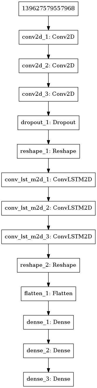
DeepestLSTM-Tinypilotnet

I’ve trained a new model: DeepestLSTM-Tinypilotnet:

model_deepestlstm_tinypilotnet