Robotics URJC
Personal webpage for TFM Students.
View the Project on GitHub RoboticsLabURJC/2017-tfm-vanessa-fernandez
Week 23: Driving videos, Pilotnet multiple (stacked), Metrics table, Basic LSTM
Driving videos
Pilotnet network [whole image]
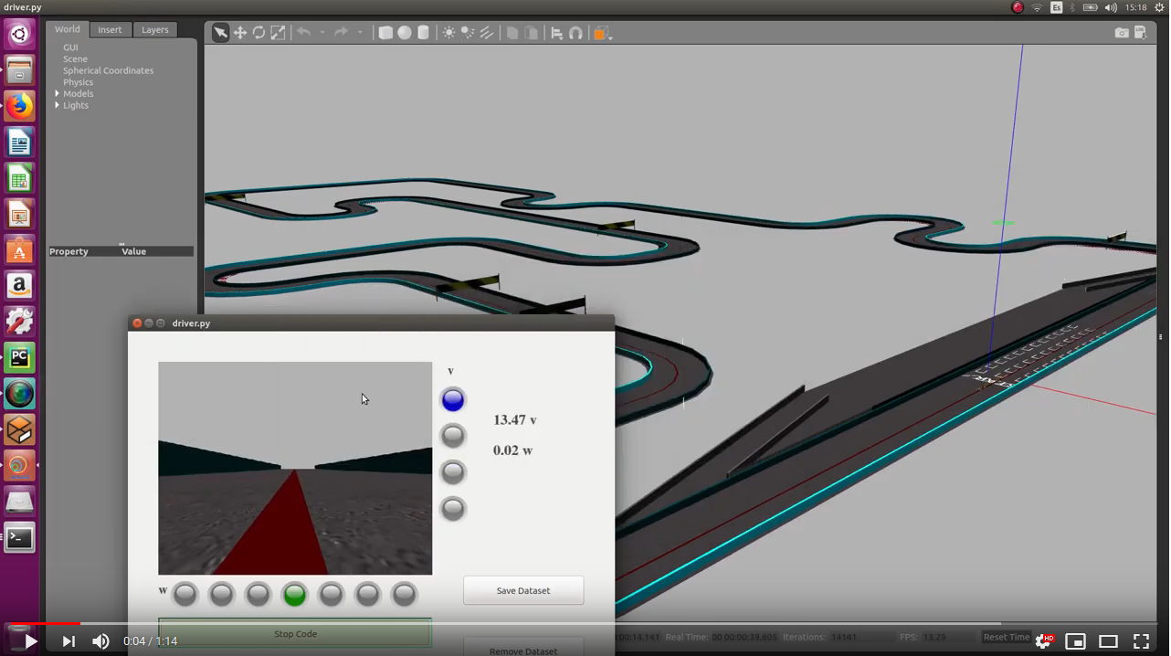
I’ve used the predictions of the Pilotnet network (regression network) to driving a formula 1 (test3):
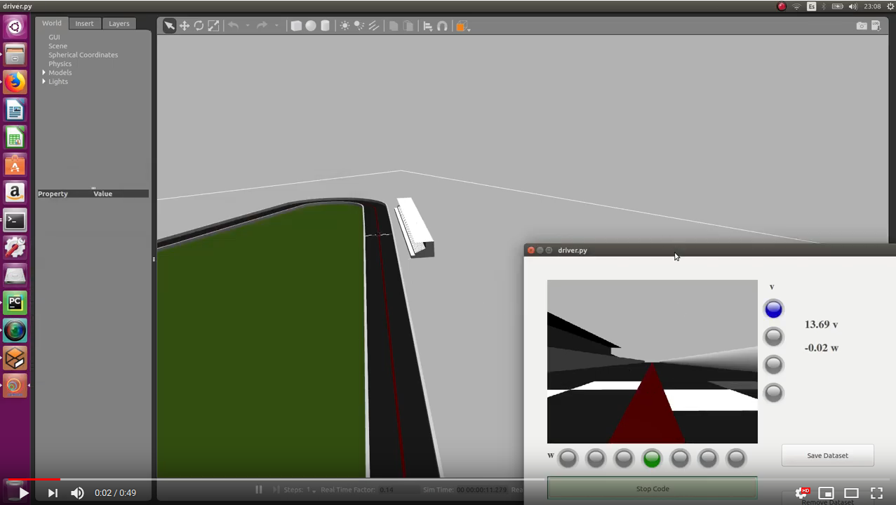
- Simple circuit clockwise (simulation time: 1min 41s):
- Simple circuit anti-clockwise (simulation time: 1min 39s):
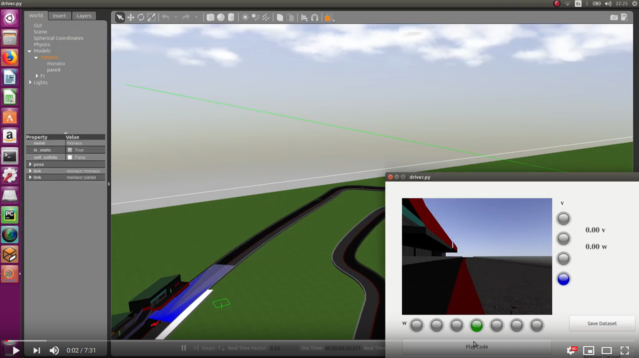
- Monaco circuit clockwise (simulation time: 1min 21s):
- Monaco circuit anti-clockwise (simulation time: 1min 23s):
- Nurburgrin circuit clockwise (simulation time: 1min 03s):
- Nurburgrin circuit anti-clockwise (simulation time: 1min 06s):
Tinypilotnet network [whole image]
I’ve used the predictions of the Tinypilotnet network (regression network) to driving a formula 1:
- Simple circuit clockwise (simulation time: 1min 39s):
- Simple circuit anti-clockwise (simulation time: 1min 38s):
- Monaco circuit clockwise (simulation time: 1min 19s):
- Monaco circuit anti-clockwise (simulation time: 1min 20s):
- Nurburgrin circuit clockwise (simulation time: 1min 05s):
- Nurburgrin circuit anti-clockwise (simulation time: 1min 06s):
Biased classfication network [cropped image]
I’ve used the predictions of the classification network according to w (7 classes) and v (4 classes) to driving a formula 1 (simulation time: 1min 38s):
Results table (cropped image)
| Driving results (regression networks) | ||||||||||||||
| Manual | Pilotnet v + w | TinyPilotnet v + w | Stacked v+w | Stacked (diff) v+w | LSTM-Tinypilotnet v + w | DeepestLSTM-Tinypilot. | ||||||||
| Circuits | Percentage | Time | Percentage | Time | Percentage | Time | Percentage | Time | Percentage | Time | Percentage | Time | Percentage | Time |
| Simple (clockwise) | 100% | 1min 35s | 100% | 1min 40s | 100% | 1min 40s | 100% | 1min 41s | 100% | 1min 39s | 100% | 1min 40s | 100% | 1min 37s |
| Simple (anti-clockwise) | 100% | 1min 32s | 100% | 1min 45s | 100% | 1min 40s | 10% | 100% | 1min 38s | 100% | 1min 38s | 100% | 1min 38s | |
| Monaco (clockwise) | 100% | 1min 15s | 85% | 85% | 85% | 45% | 50% | 55% | ||||||
| Monaco (anti-clockwise) | 100% | 1min 15s | 100% | 1min 20s | 100% | 1min 18s | 15% | 5% | 35% | 55% | ||||
| Nurburgrin (clockwise) | 100% | 1min 02s | 100% | 1min 04s | 100% | 1min 04s | 8% | 8% | 40% | 100% | 1min 04s | |||
| Nurburgrin (anti-clockwise) | 100% | 1min 02s | 100% | 1min 05s | 100% | 1min 05s | 80% | 50% | 50% | 80% |
| Driving results (classification networks) | ||||||||||||||
| Manual | 1v+7w biased | 4v+7w biased | 1v+7w balanced | 4v+7w balanced | 1v+7w imbalanced | 4v+7w imbalanced | ||||||||
| Circuits | Percentage | Time | Percentage | Time | Percentage | Time | Percentage | Time | Percentage | Time | Percentage | Time | Percentage | Time |
| Simple (clockwise) | 100% | 1min 35s | 100% | 2min 16s | 100% | 1min 38s | 100% | 2min 16s | 98% | 100% | 2min 16s | 100% | 1min 42s | |
| Simple (anti-clockwise) | 100% | 1min 32s | 100% | 2min 16s | 100% | 1min 38s | 100% | 2min 16s | 100% | 1min 41s | 100% | 2min 16s | 100% | 1min 39s |
| Monaco (clockwise) | 100% | 1min 15s | 45% | 5% | 5% | 5% | 5% | 5% | ||||||
| Monaco (anti-clockwise) | 100% | 1min 15s | 15% | 5% | 5% | 5% | 5% | 5% | ||||||
| Nurburgrin (clockwise) | 100% | 1min 02s | 8% | 8% | 8% | 8% | 8% | 8% | ||||||
| Nurburgrin (anti-clockwise) | 100% | 1min 02s | 80% | 90% | 80% | 80% | 80% | 80% |
Results table (whole image)
| Driving results (regression networks) | ||||||||||||||
| Manual | Pilotnet v + w | TinyPilotnet v + w | Stacked v+w | Stacked (diff) v+w | LSTM-Tinypilotnet v + w | DeepestLSTM-Tinypilot. | ||||||||
| Circuits | Percentage | Time | Percentage | Time | Percentage | Time | Percentage | Time | Percentage | Time | Percentage | Time | Percentage | Time |
| Simple (clockwise) | 100% | 1min 35s | 100% | 1min 41s | 100% | 1min 39s | 100% | 1min 40s | 100% | 1min 43s | 100% | 1min 39s | 100% | 1min 39s |
| Simple (anti-clockwise) | 100% | 1min 32s | 100% | 1min 39s | 100% | 1min 38s | 100% | 1min 46s | 10% | 10% | 100% | 1min 41s | ||
| Monaco (clockwise) | 100% | 1min 15s | 100% | 1min 21s | 100% | 1min 19s | 50% | 5% | 100% | 1min 27s | 50% | |||
| Monaco (anti-clockwise) | 100% | 1min 15s | 100% | 1min 23s | 100% | 1min 20s | 7% | 5% | 50% | 100% | 1min 21s | |||
| Nurburgrin (clockwise) | 100% | 1min 02s | 100% | 1min 03s | 100% | 1min 05s | 50% | 8% | 100% | 1min 08s | 100% | 1min 05s | ||
| Nurburgrin (anti-clockwise) | 100% | 1min 02s | 100% | 1min 06s | 100% | 1min 06s | 80% | 50% | 50% | 100% | 1min 07s |
| Driving results (classification networks) | ||||||||||||||
| Manual | 1v+7w biased | 4v+7w biased | 1v+7w balanced | 4v+7w balanced | 1v+7w imbalanced | 4v+7w imbalanced | ||||||||
| Circuits | Percentage | Time | Percentage | Time | Percentage | Time | Percentage | Time | Percentage | Time | Percentage | Time | Percentage | Time |
| Simple (clockwise) | 100% | 1min 35s | 100% | 2min 17s | 70% | 75% | 7% | 100% | 2min 17s | 40% | ||||
| Simple (anti-clockwise) | 100% | 1min 32s | 100% | 2min 17s | 10% | 100% | 2min 16s | 7% | 100% | 2min 16s | 10% | |||
| Monaco (clockwise) | 100% | 1min 15s | 5% | 5% | 5% | 5% | 5% | 5% | ||||||
| Monaco (anti-clockwise) | 100% | 1min 15s | 5% | 5% | 5% | 5% | 5% | 5% | ||||||
| Nurburgrin (clockwise) | 100% | 1min 02s | 8% | 8% | 8% | 8% | 8% | 8% | ||||||
| Nurburgrin (anti-clockwise) | 100% | 1min 02s | 8% | 8% | 8% | 8% | 8% | 8% |
Pilotnet multiple (stacked)
In this method (stacked frames), we concatenate multiple subsequent input images to create a stacked image. Then, we feed this stacked image to the network as a single input. In this case, we have stacked 2 images separated by 10 frames. The results are:
| Driving results (regression networks) | ||||||||
| stacked const v whole image | stacked whole image | stacked const v cropped image | stacked cropped image | |||||
| Circuits | Percentage | Time | Percentage | Time | Percentage | Time | Percentage | Time |
| Simple (clockwise) | 100% | 3min 45s | 100% | 1min 40s | 100% | 3min 46s | 100% | 1min 41s |
| Simple (anti-clockwise) | 100% | 3min 47s | 100% | 1min 46s | 100% | 3min 46s | 10% | |
| Monaco (clockwise) | 100% | 2min 56s | 50% | 100% | 2min 56s | 85% | ||
| Monaco (anti-clockwise) | 7% | 7% | 7% | 15% | ||||
| Nurburgrin (clockwise) | 8% | 50% | 8% | 8% | ||||
| Nurburgrin (anti-clockwise) | 100% | 2min 27s | 80% | 90% | 80% |
We have also tried to stack 2 images, but separated but one is the image in the instantaneous it and the other is the difference image of it and it-10. The results are:
| Driving results (regression networks) | ||||||||
| stacked const v whole image | stacked whole image | stacked const v cropped image | stacked cropped image | |||||
| Circuits | Percentage | Time | Percentage | Time | Percentage | Time | Percentage | Time |
| Simple (clockwise) | 100% | 3min 45s | 100% | 1min 43s | 100% | 3min 46s | 100% | 1min 39s |
| Simple (anti-clockwise) | 100% | 3min 36s | 10% | 100% | 3min 46s | 100% | 1min 38s | |
| Monaco (clockwise) | 45% | 5% | 50% | 45% | ||||
| Monaco (anti-clockwise) | 5% | 5% | 7% | 5% | ||||
| Nurburgrin (clockwise) | 8% | 8% | 8% | 8% | ||||
| Nurburgrin (anti-clockwise) | 90% | 50% | 90% | 50% |
Metrics table (cropped image)
- Metrics results (Classification networks) (Train data):
| Classification 7w biased | Classification 4v biased | ||||||||
| Accuracy | Accuracy top 2 | Precision | Recall | F1-score | Accuracy | Accuracy top 2 | Precision | Recall | F1-score |
| 97% | 99% | 98% | 97% | 97% | 98% | 99% | 98% | 98% | 98% |
| Classification 7w balanced | Classification 4v balanced | ||||||||
| Accuracy | Accuracy top 2 | Precision | Recall | F1-score | Accuracy | Accuracy top 2 | Precision | Recall | F1-score |
| 95% | 99% | 96% | 95% | 95% | 94% | 97% | 95% | 95% | 95% |
| Classification 7w imbalanced | Classification 4v bimbalanced | ||||||||
| Accuracy | Accuracy top 2 | Precision | Recall | F1-score | Accuracy | Accuracy top 2 | Precision | Recall | F1-score |
| 98% | 99% | 99% | 99% | 99% | 98% | 99% | 98% | 98% | 98% |
- Metrics results (Classification networks) (Test data):
| Classification 7w biased | Classification 4v biased | ||||||||
| Accuracy | Accuracy top 2 | Precision | Recall | F1-score | Accuracy | Accuracy top 2 | Precision | Recall | F1-score |
| 94% | 99% | 95% | 95% | 95% | 95% | 98% | 95% | 95% | 95% |
| Classification 7w balanced | Classification 4v balanced | ||||||||
| Accuracy | Accuracy top 2 | Precision | Recall | F1-score | Accuracy | Accuracy top 2 | Precision | Recall | F1-score |
| 93% | 99% | 94% | 94% | 94% | 92% | 96% | 94% | 93% | 93% |
| Classification 7w imbalanced | Classification 4v bimbalanced | ||||||||
| Accuracy | Accuracy top 2 | Precision | Recall | F1-score | Accuracy | Accuracy top 2 | Precision | Recall | F1-score |
| 95% | 99% | 95% | 95% | 95% | 95% | 97% | 95% | 95% | 95% |
- Metrics results (Regression networks) (Train data):
| Pilotnet w | Pilotnet v | Pilotnet w multiple (stacked) | Pilotnet v multiple (stacked) | ||||
| Mean squared error | Mean absolute error | Mean squared error | Mean absolute error | Mean squared error | Mean absolute error | Mean squared error | Mean absolute error |
| 0.001754 | 0.027871 | 0.626956 | 0.452977 | 0.110631 | 0.230633 | 5.215044 | 1.563034 |
- Metrics results (Regression networks) (Test data):
| Pilotnet w | Pilotnet v | Pilotnet w multiple (stacked) | Pilotnet v multiple (stacked) | ||||
| Mean squared error | Mean absolute error | Mean squared error | Mean absolute error | Mean squared error | Mean absolute error | Mean squared error | Mean absolute error |
| 0.002206 | 0.030515 | 0.849241 | 0.499219 | 0.108316 | 0.226848 | 5.272124 | 1.552658 |
Metrics table (whole image)
- Metrics results (Classification networks) (Train data):
| Classification 7w biased | Classification 4v biased | ||||||||
| Accuracy | Accuracy top 2 | Precision | Recall | F1-score | Accuracy | Accuracy top 2 | Precision | Recall | F1-score |
| 97% | 99% | 97% | 97% | 97% | 97% | 99% | 98% | 98% | 98% |
| Classification 7w balanced | Classification 4v balanced | ||||||||
| Accuracy | Accuracy top 2 | Precision | Recall | F1-score | Accuracy | Accuracy top 2 | Precision | Recall | F1-score |
| 95% | 99% | 96% | 96% | 96% | 90% | 95% | 90% | 90% | 90s% |
| Classification 7w imbalanced | Classification 4v bimbalanced | ||||||||
| Accuracy | Accuracy top 2 | Precision | Recall | F1-score | Accuracy | Accuracy top 2 | Precision | Recall | F1-score |
| 98% | 99% | 98% | 98% | 98% | 96% | 98% | 96% | 96% | 96% |
- Metrics results (Classification networks) (Test data):
| Classification 7w biased | Classification 4v biased | ||||||||
| Accuracy | Accuracy top 2 | Precision | Recall | F1-score | Accuracy | Accuracy top 2 | Precision | Recall | F1-score |
| 95% | 99% | 95% | 95% | 95% | 94% | 97% | 95% | 95% | 95% |
| Classification 7w balanced | Classification 4v balanced | ||||||||
| Accuracy | Accuracy top 2 | Precision | Recall | F1-score | Accuracy | Accuracy top 2 | Precision | Recall | F1-score |
| 93% | 99% | 94% | 93% | 93% | 89% | 95% | 91% | 89% | 90% |
| Classification 7w imbalanced | Classification 4v bimbalanced | ||||||||
| Accuracy | Accuracy top 2 | Precision | Recall | F1-score | Accuracy | Accuracy top 2 | Precision | Recall | F1-score |
| 95% | 99% | 95% | 95% | 95% | 94% | 97% | 95% | 95% | 95% |
- Metrics results (Regression networks) (Train data):
| Pilotnet w | Pilotnet v | Stacked w | Stacked v | DeepestLSTM-Tinypilotnet w | DeepestLSTM-Tinypilotnet v | ||||||
| MSE | MAE | MSE | MAE | MSE | MAE | MSE | MAE | MSE | MAE | MSE | MAE |
| 0.000660 | 0.015514 | 0.809848 | 0.548209 | 0.068739 | 0.167565 | 8.973208 | 1.997035 | 1.997035 | 0.021000 | 0.491759 | 0.383216 |
- Metrics results (Regression networks) (Test data):
| Pilotnet w | Pilotnet v | Stacked w | Stacked v | DeepestLSTM-Tinypilotnet w | DeepestLSTM-Tinypilotnet v | ||||||
| MSE | MAE | MSE | MAE | MSE | MAE | MSE | MAE | MSE | MAE | MSE | MAE |
| 0.000938 | 0.017433 | 1.374714 | 0.659400 | 0.067305 | 0.164354 | 9.402403 | 2.039585 | 0.000982 | 0.020472 | 0.549310 | 0.399267 |
Basic CNN+LSTM
I have created a network cnn + lstm and I have trained it with a set of 10 images. There are very few data, but so I tested the network that did not work with the original dataset.The code is:
import glob
import cv2
import numpy as np

from time import time
from matplotlib import pyplot as plt
from sklearn.model_selection import train_test_split

from keras.models import Sequential
from keras.layers import Flatten, Dense, Conv2D, BatchNormalization, Dropout, Reshape, MaxPooling2D, Activation
from keras.layers.recurrent import LSTM
from keras.optimizers import Adam


def get_images(list_images):
    # We read the images
    array_imgs = []
    for name in list_images:
        img = cv2.imread(name)
        img = cv2.resize(img, (img.shape[1] / 6, img.shape[0] / 6))
        array_imgs.append(img)

    return array_imgs


def lstm_model(img_shape):
    model = Sequential()

    model.add(Conv2D(32, (3, 3), padding='same', input_shape=img_shape, activation="relu"))
    model.add(BatchNormalization(axis=-1))
    model.add(MaxPooling2D(pool_size=(3, 3)))
    model.add(Dropout(0.25))

    model.add(Conv2D(64, (3, 3), padding='same', activation="relu"))
    model.add(BatchNormalization(axis=-1))
    model.add(Conv2D(64, (3, 3), padding='same', activation="relu"))
    model.add(BatchNormalization(axis=-1))
    model.add(MaxPooling2D(pool_size=(2, 2)))
    model.add(Dropout(0.25))

    model.add(Conv2D(128, (3, 3), padding='same', activation="relu"))
    model.add(BatchNormalization(axis=-1))
    model.add(Conv2D(128, (3, 3), padding='same', activation="relu"))
    model.add(BatchNormalization(axis=-1))
    model.add(MaxPooling2D(pool_size=(2, 2)))
    model.add(Dropout(0.25))

    model.add(Flatten())
    model.add(Dense(1024))
    model.add(Activation('relu'))
    model.add(BatchNormalization())
    model.add(Dropout(0.5))

    model.add(Reshape((1024, 1)))
    model.add(LSTM(10, return_sequences = True))
    model.add(Dropout(0.2))
    model.add(LSTM(10))
    model.add(Dropout(0.2))
    model.add(Dense(5, activation="relu"))
    model.add(Dense(1))
    adam = Adam(lr=0.0001)
    model.compile(optimizer=adam, loss="mse", metrics=['accuracy', 'mse', 'mae'])
    return model


if __name__ == "__main__":

    # Load data
    list_images = glob.glob('Images/' + '*')
    images = sorted(list_images, key=lambda x: int(x.split('/')[1].split('.png')[0]))

    y = [71.71, 56.19, -44.51, 61.90, 67.86, -61.52, -75.73, 44.75, -89.51, 44.75]
    # We preprocess images
    x = get_images(images)

    X_train = x
    y_train = y
    X_t, X_val, y_t, y_val = train_test_split(x, y, test_size=0.20, random_state=42)

    # Variables
    batch_size = 8
    nb_epoch = 200
    img_shape = (39, 53, 3)


    # We adapt the data
    X_train = np.stack(X_train, axis=0)
    y_train = np.stack(y_train, axis=0)
    X_val = np.stack(X_val, axis=0)
    y_val = np.stack(y_val, axis=0)


    # Get model
    model = lstm_model(img_shape)

    model_history_v = model.fit(X_train, y_train, epochs=nb_epoch, batch_size=batch_size, verbose=2,
                              validation_data=(X_val, y_val))
    print(model.summary())


    # We evaluate the model
    score = model.evaluate(X_val, y_val, verbose=0)
    print('Evaluating')
    print('Test loss: ', score[0])
    print('Test accuracy: ', score[1])
    print('Test mean squared error: ', score[2])
    print('Test mean absolute error: ', score[3])
The results are:
_________________________________________________________________
Layer (type)                 Output Shape              Param #
=================================================================
conv2d_1 (Conv2D)            (None, 39, 53, 32)        896
_________________________________________________________________
batch_normalization_1 (Batch (None, 39, 53, 32)        128
_________________________________________________________________
max_pooling2d_1 (MaxPooling2 (None, 13, 17, 32)        0
_________________________________________________________________
dropout_1 (Dropout)          (None, 13, 17, 32)        0
_________________________________________________________________
conv2d_2 (Conv2D)            (None, 13, 17, 64)        18496
_________________________________________________________________
batch_normalization_2 (Batch (None, 13, 17, 64)        256
_________________________________________________________________
conv2d_3 (Conv2D)            (None, 13, 17, 64)        36928
_________________________________________________________________
batch_normalization_3 (Batch (None, 13, 17, 64)        256
_________________________________________________________________
max_pooling2d_2 (MaxPooling2 (None, 6, 8, 64)          0
_________________________________________________________________
dropout_2 (Dropout)          (None, 6, 8, 64)          0
_________________________________________________________________
conv2d_4 (Conv2D)            (None, 6, 8, 128)         73856
_________________________________________________________________
batch_normalization_4 (Batch (None, 6, 8, 128)         512
_________________________________________________________________
conv2d_5 (Conv2D)            (None, 6, 8, 128)         147584
_________________________________________________________________
batch_normalization_5 (Batch (None, 6, 8, 128)         512
_________________________________________________________________
max_pooling2d_3 (MaxPooling2 (None, 3, 4, 128)         0
_________________________________________________________________
dropout_3 (Dropout)          (None, 3, 4, 128)         0
_________________________________________________________________
flatten_1 (Flatten)          (None, 1536)              0
_________________________________________________________________
dense_1 (Dense)              (None, 1024)              1573888
_________________________________________________________________
activation_1 (Activation)    (None, 1024)              0
_________________________________________________________________
batch_normalization_6 (Batch (None, 1024)              4096
_________________________________________________________________
dropout_4 (Dropout)          (None, 1024)              0
_________________________________________________________________
reshape_1 (Reshape)          (None, 1024, 1)           0
_________________________________________________________________
lstm_1 (LSTM)                (None, 1024, 10)          480
_________________________________________________________________
dropout_5 (Dropout)          (None, 1024, 10)          0
_________________________________________________________________
lstm_2 (LSTM)                (None, 10)                840
_________________________________________________________________
dropout_6 (Dropout)          (None, 10)                0
_________________________________________________________________
dense_2 (Dense)              (None, 5)                 55
_________________________________________________________________
dense_3 (Dense)              (None, 1)                 6
=================================================================
Total params: 1,858,789
Trainable params: 1,855,909
Non-trainable params: 2,880
_________________________________________________________________
None
Evaluating
('Test loss: ', 5585.3828125)
('Test accuracy: ', 0.0)
('Test mean squared error: ', 5585.3828125)
('Test mean absolute error: ', 72.8495864868164)
from keras.preprocessing import sequence from keras.models import Sequential from keras.layers import Dense, Dropout, Embedding, LSTM from keras.datasets import imdb
We load dataset of top 1000 words
num_words = 1000 (X_train, y_train), (X_test, y_test) = imdb.load_data(num_words=num_words)
We need to divide this dataset and create and pad sequences (using sequence from keras.preprocessing)
In the padding we used number 200, meaning that our sequences will be 200 words long
X_train = sequence.pad_sequences(X_train, maxlen=200) X_test = sequence.pad_sequences(X_test, maxlen=200)
Define network architecture and compile
model = Sequential() model.add(Embedding(num_words, 50, input_length=200)) model.add(Dropout(0.2)) model.add(LSTM(100, dropout=0.2, recurrent_dropout=0.2)) model.add(Dense(250, activation=’relu’)) model.add(Dropout(0.2)) model.add(Dense(1, activation=’sigmoid’)) model.compile(loss=’binary_crossentropy’, optimizer=’adam’, metrics=[‘accuracy’])
We train the model
model.fit(X_train, y_train, batch_size=64, epochs=15)
We evaluate the model
score = model.evaluate(X_test, y_test) print(‘Test loss:’, score[0]) print(‘Test accuracy:’, score[1]) </pre>
We got the accuracy of 86.42%.
ETA: 0s - loss: 0.2874 - acc: 0.825000/25000 [==============================] - 134s 5ms/step - loss: 0.2875 - acc: 0.8776
25000/25000 [==============================] - 47s 2ms/step
('Test loss:', 0.32082191239356994)
('Test accuracy:', 0.86428)
Basic LSTM
I’ve followed a LSTM tutorial to create an LSTM network in Keras. We’ve classified reviews from the IMDB dataset. The LSTM networks aren’t keeping just propagating output information to the next time step, but they are also storing and propagating the state of the so-called LSTM cell. This cell is holding four neural networks inside – gates, which are used to decide which information will be stored in cell state and pushed to output. So, the output of the network at one time step is not depending only on the previous time step but depends on n previous time steps.
The dataset was collected by Stanford researchers back in 2011. It contains 25000 movie reviews (good or bad) for training and the same amount of reviews for testing. Our goal is to create a network that will be able to determine which of these reviews are positive and which are negative. Words are encoded as real-valued vectors in a high dimensional space, where the similarity between words in terms of meaning translates to closeness in the vector space.
The code is the following: