Comparing Pilotnet vs Deepest LSTM TinyPilotNet using Behavior Metrics

We will be comparing two approaches that are currently giving good results on the different circuits that are part of Behavior Metrics. The metrics used are objective, extracted from Behavior Metrics, the tool that we use for running and testing the brains that retireves actual metrics of the performance and we will be understanding the results that it retrieves.

The brains for comparison are PilotNet and Deepest LSTM TinyPilotNet, two brain architectures based on deep learning that we have been studying and testing for our problems for a while.

We will first explore how the training has been conducted, since for these two approaches there are some differences on that process. The first approach, PilotNet, is an instantaneous architecture, without temporal information, that returns 2 speeds (linear and angular) from an image that pass through it. In contrast, Deepest TinyPilotNet’s architecture as a different key component on its inside, some LSTM cells. These cells are useful for scenarios where the temporal information is relevant. In our case, since the we are dealing with the problem of driving, the temporal factor should be relevant somehow.

Let’s see how we have trained these two brains!

Training PilotNet

For this first architecture, we prepare the image data for training as follows:

1. We use the complete_dataset already separated folders Train and Test.
2. The images are cropped on the horizon line because the upper information only adds noise but is not relevant for this scenario.
3. These images are additionally flipped on a pretraining stage
4. We add repeated examples to the dataset taking into consideration extreme cases. A extrema case is when the value for the W, which can be [-3, 3] is on case 1 [>1,<-1] or case 2 [>2,<-2]. Depending on how extreme the case is (case 1 or case 2) it is added more times. Same for the V [0, 13], when a extreme case appears [<2] it’s added more times.
5. After this stage, the dataset is normalized for the annotations.
6. The dataset is divided in train-val shuffling the data.
7. This dataset is trained using the PilotNet architecture combining different probabilistic augmentations using albumentations library. The agumentations are: RandomBrightnessContrast, HueSaturationValue, FancyPCA, RandomGamma, GaussianBlur, GaussNoise and Normalize.
8. A batch size of 50 and 100 epochs are used with a 0.0001 learning rate and images of size (200,66).

Training Deepest LSTM TinyPilotNet

For the second architecture, the data preparation is:

1. In this case instead of using directly the prepared folders, we use the complete_dataset and curves_only folder. This change is mandatory because the prepared folders come with the images shuffled and me need sequences for this case (we need to keep the temporal dependency of the data.)
2. Again, the images are cropped on the horizon and then flipped.
3. The data now is separated on its actual sequences divisible by 50. The dataset comes with many sequences of different length so we get rid of some images to make every sequence length divisible by 50.
4. After this, we add the extreme mini sequences (divisible by 50) of every sequence several times to balance the data. This is done repeating the sequences that are extreme based on the same criteria used on PilotNet.
5. These sequences are then shuffled between them but conserving the sequence nature (temporal factor).
6. The data is splitted between train-val but without shuffling, not to lose the temporal information.
7. The training is conducted, combining the same probabilistic augmentations on the data but in this case instead of applying different agumentations for every image on the batch, the same augmentation is applied on the whole batch, again not to lose the temporal information.
8. The network is trained once again on the same manner than PilotNet but with a image size of [100,50].

Results

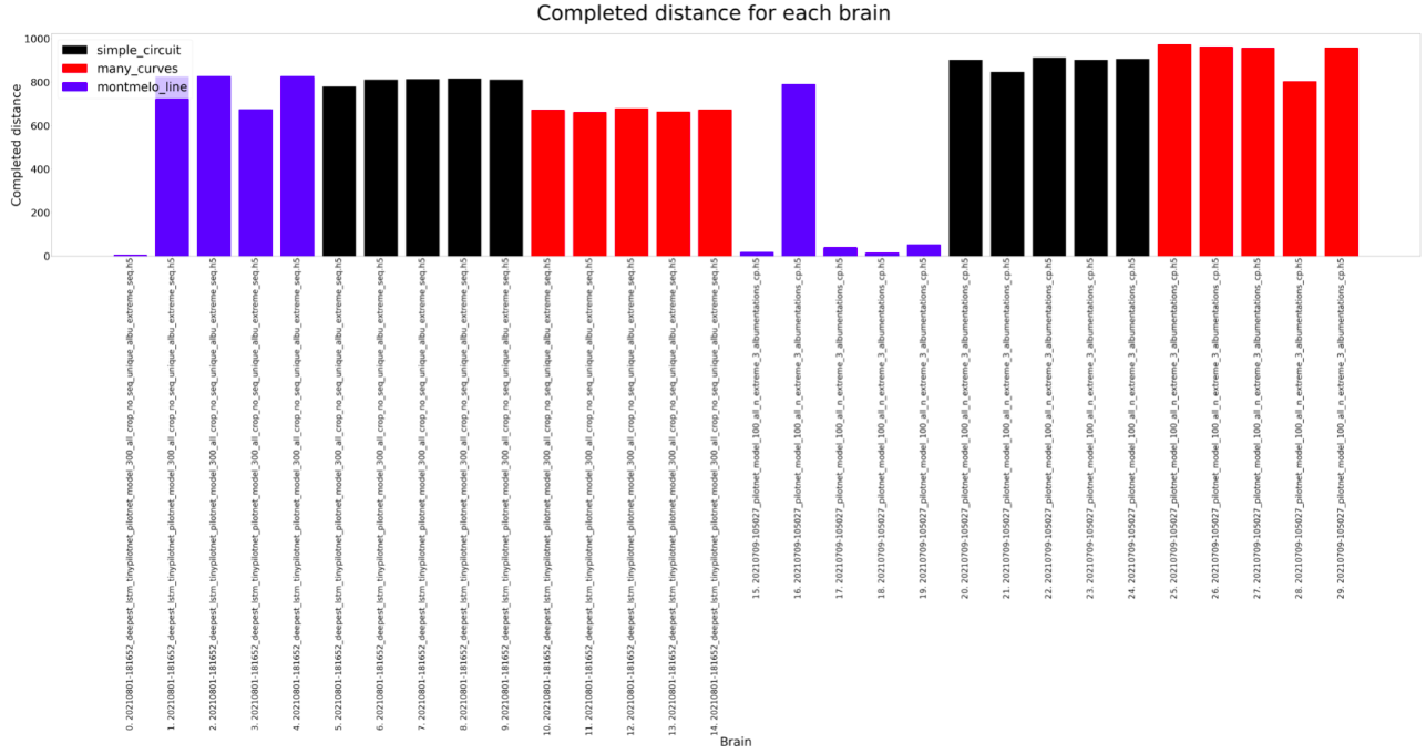
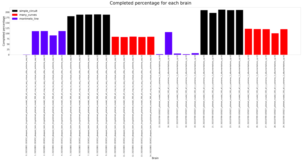
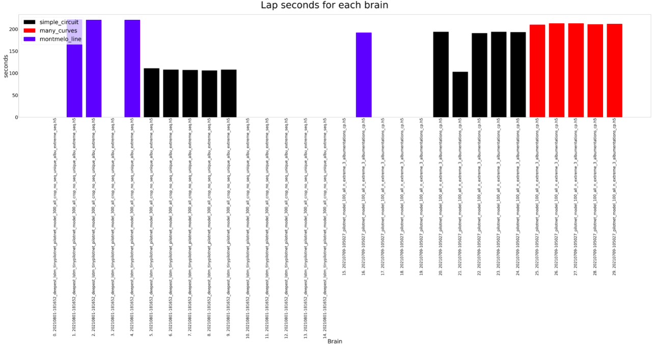
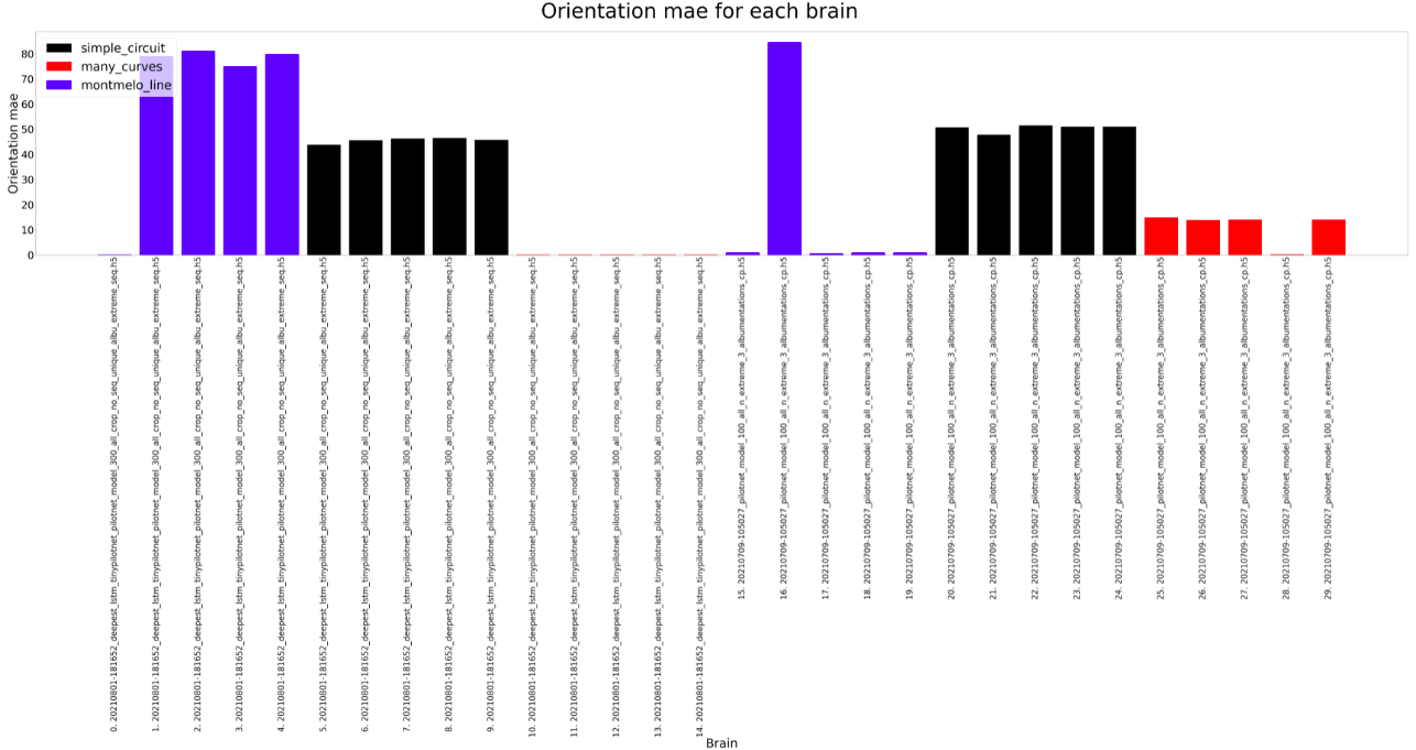
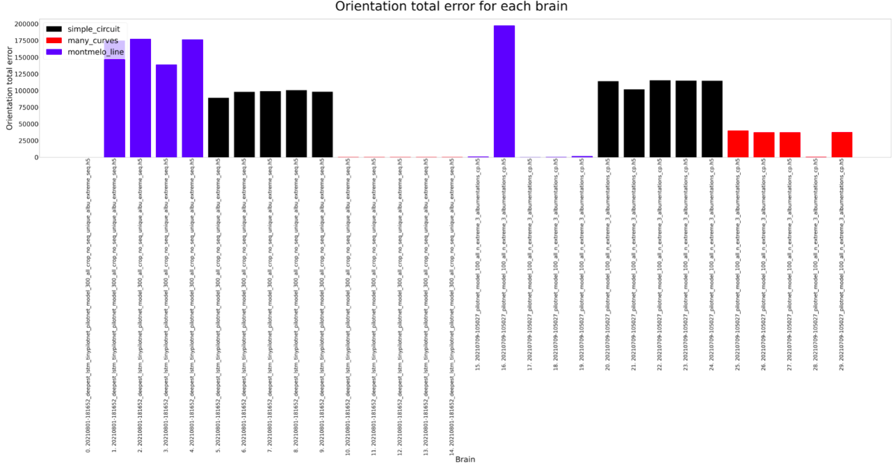
For the experiment, each brain is ran on every circuit (Simple, many curves and montmeló) 5 times for the estimated duration of a lap on that brain (200, 250, 200). Considering that, the results can be shown below. As we can see on the plots, the results are similar, both can complete all the circuits, but there are some differences.

The Deepest LSTM TinyPilotnet (LSTM brain for short) finishes always all the different circuits. The completed distance is slightly higher for the PilotNet brain, so it seems that the LSTM brain learns not to run fast. The completed percentage follows the same idea. The orientation MAE and total error is higher on the PilotNet brain, which could be due to the higher speed of this brain, which leads to more non-precise predictions. Finally, the lap seconds show that for Montmeló PilotNet is faster but the rest of the results are a bit weird, something that should be explored.