Learning to drive with deep learning. Experiments with 4 types of nets and comparison

In this blogpost, I will sum up the last weeks (months) of work in this project. Many improvements have been made and my general knowledge of this huge area is now broader but still quite small.

Introduction

For this problem, we would like to generate a brain that learns to drive the circuits that we have autonomously. The brain will need to learn to generate two outputs, the speed V and the rotation W. For this purpose, we have a dataset consisting of images with annotations V, W generated from an explicit brain.

Brains

4 approaches are explored, all of them from the literature. We select previous brains used in the literature because in this phase we are only learning concepts and we are not trying to outperform the state of the art (probably that will be covered some time soon :)).

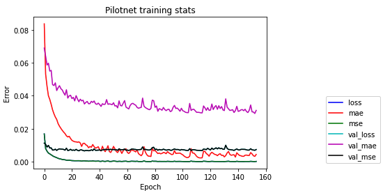
PilotNet

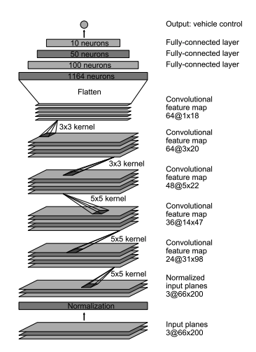
The first brain comes from two papers 1 2 proposed by Nvidia. In these papers they present a deep learning architecture called PilotNet based on a CNN that learns to drive using data from a real environment. Our case is much simpler, so this network could be a good start point to learn the concepts.

This model has 12000000 params.

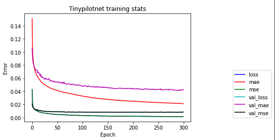
TinyPilotNet

This network and teh following ones come from the paper Self-driving a Car in Simulation Through a CNN. They present different approaches to improve the PilotNet architecture for autonomous driving using a smaller network (this case) or more advance concepts like LSTMs nodes (the following brains).

This architecture takes the same ideas from PilotNet but making the network simpler and smaller. This model has 220000 params.

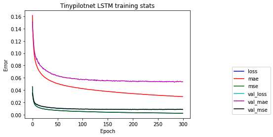
TinyPilonetNet LSTM

In this architecture, the ideas from the previous architecture are used combined with an LSTM node to learn temporal dependencies. This could make sense for the problem of autonomously driving because previous steps in time are sometime useful for current predictions (imagine taking a curve). This model has 920000 params.

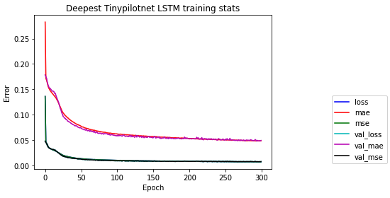
Deepest TinypilotNet LSTM

Finally, the most complex network is also based on the previous one, but adding more LSTM layers to make ir deeper and learn more temporal dependencies. This model has 86000 params.

Dataset

Considering the problem that we are trying to solve, we elaborated a dataset consisting of images and V-W pais predictions. This dataset comes from a variate set of circuits in both directions with an explicit brain. Since we have several sequences and we would like to learn temporal dependencies, we have to take this into account when preprocessing the data that is fed into the networks. If we want the LSTMs to learn temporal dependencies, the images should come as a sequence.

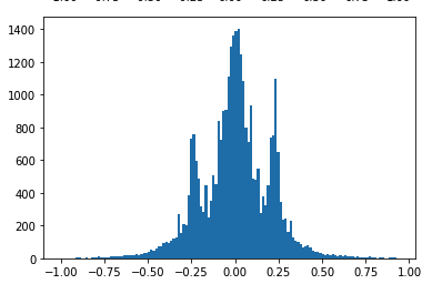
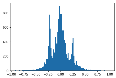
For this purpose, the data is divided into sequences that are then mixed and separated into train-val sets. Below are the distributions of data for the W value for the train and val sets.

Training

We train all of the networks with the same criteria in order to make the comparison as fair as possible. Each architecture is trained 300 epochs with batches of 50 examples. The 300 epochs are more than enough to over fit the data. On this stage that is not a problem since we are only learning concepts and the goal is to generate brains that learn to drive.

Results in test circuits

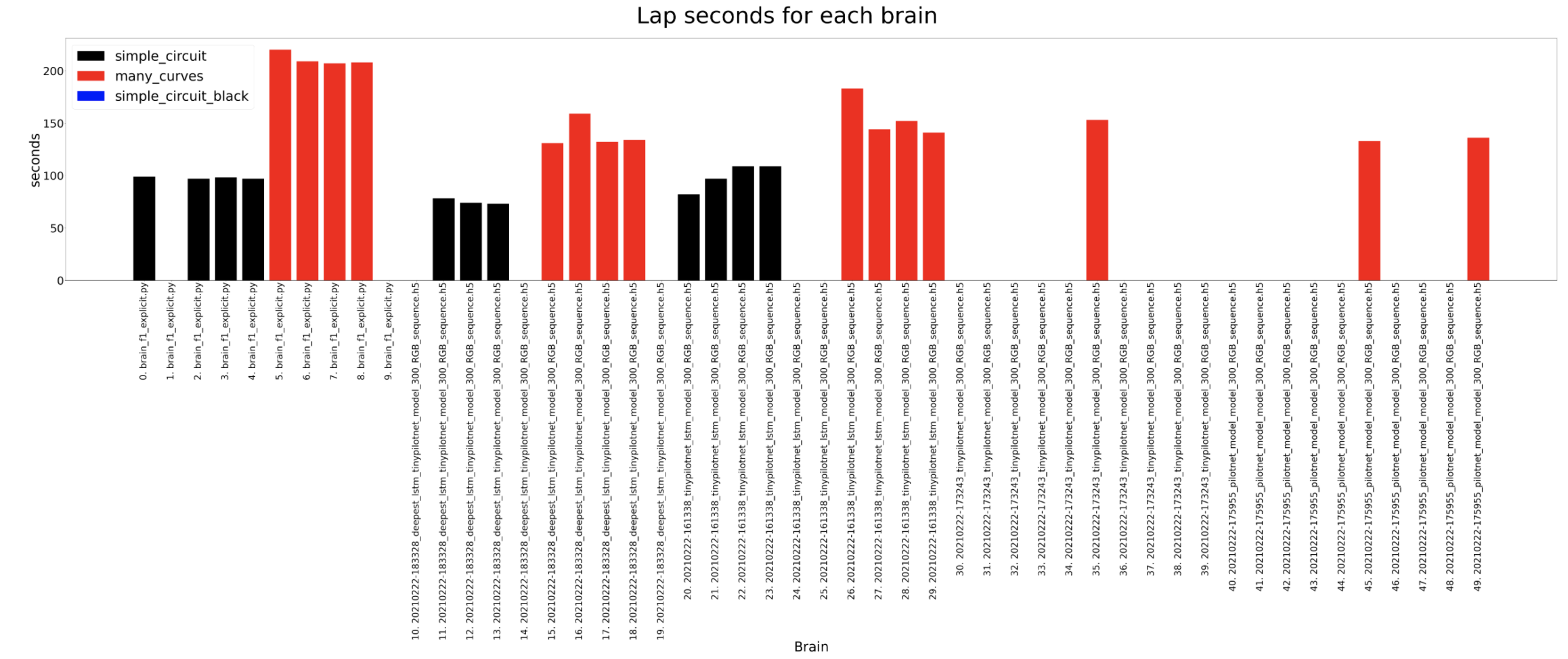
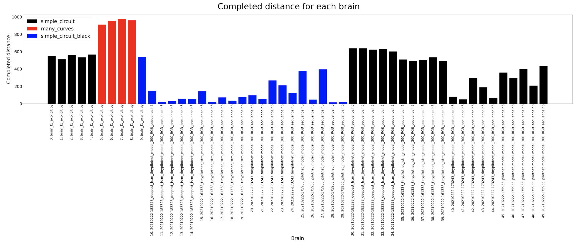
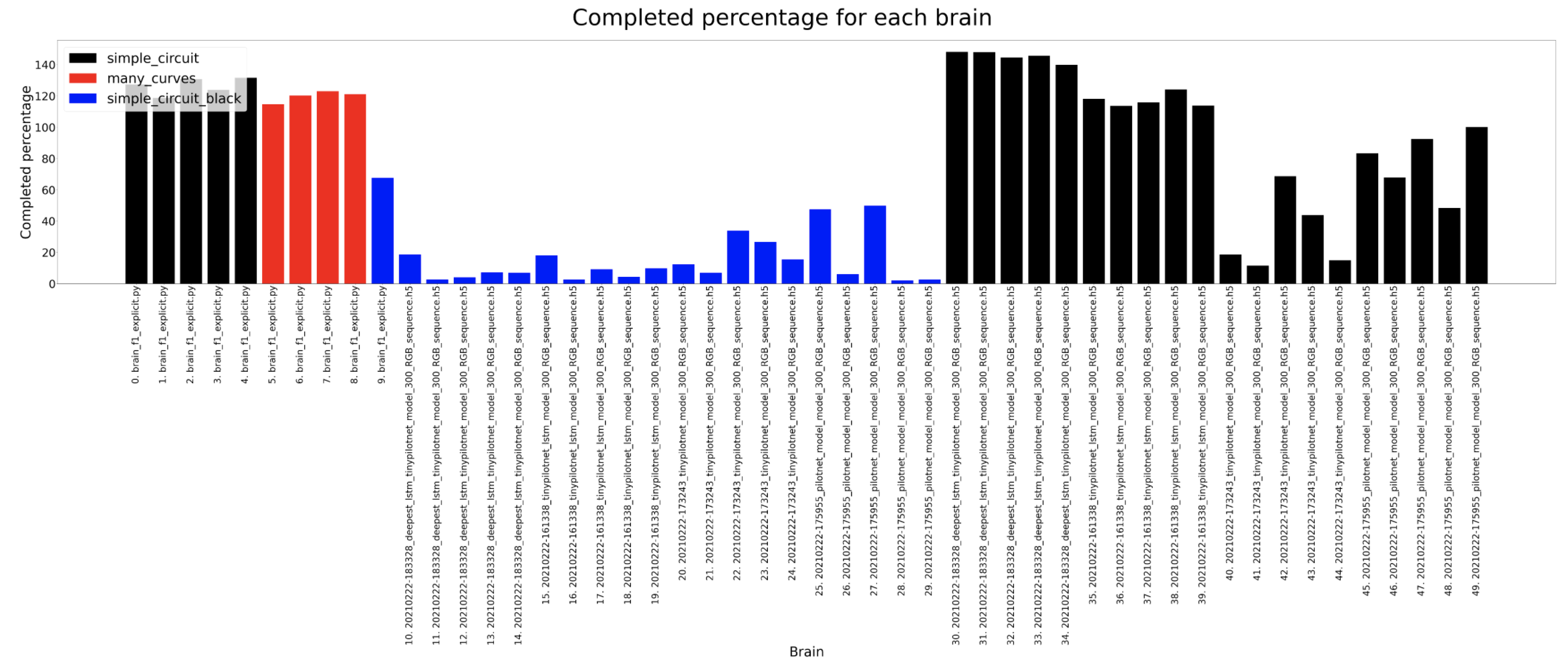
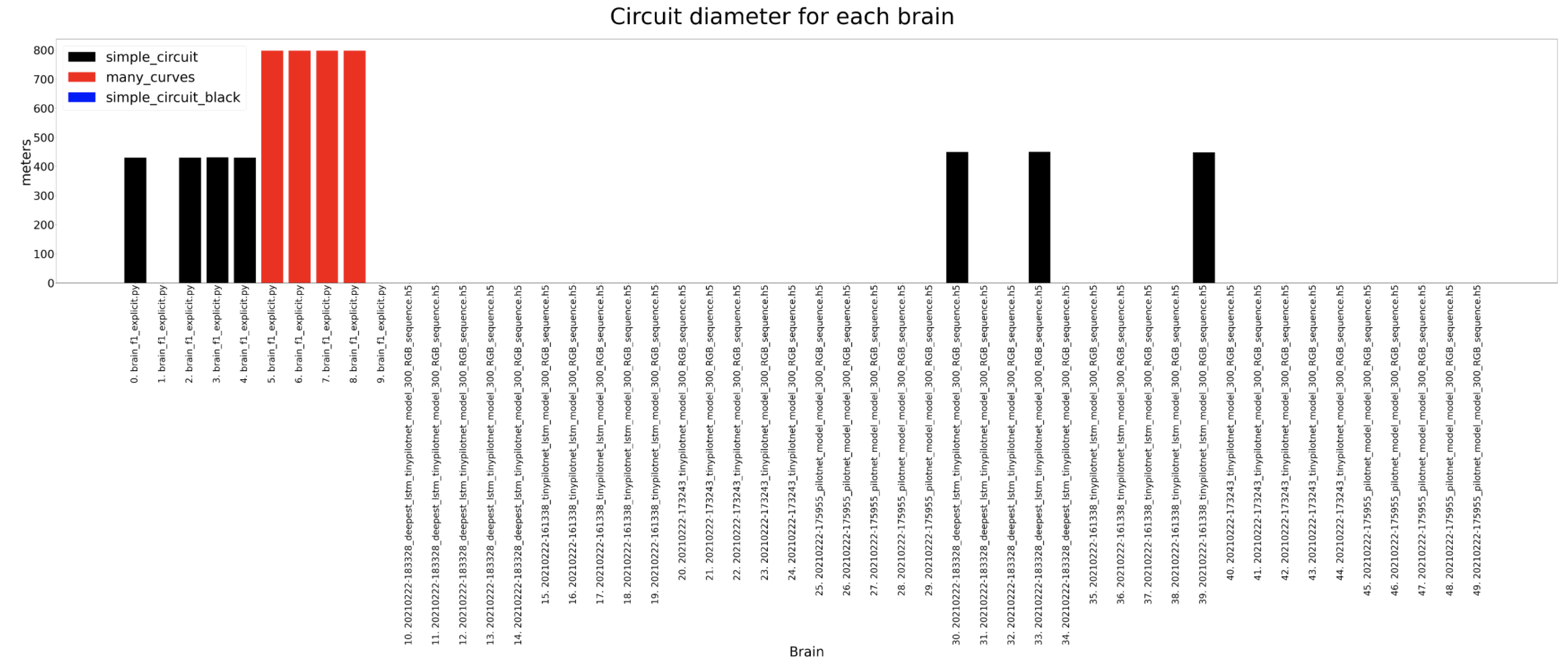
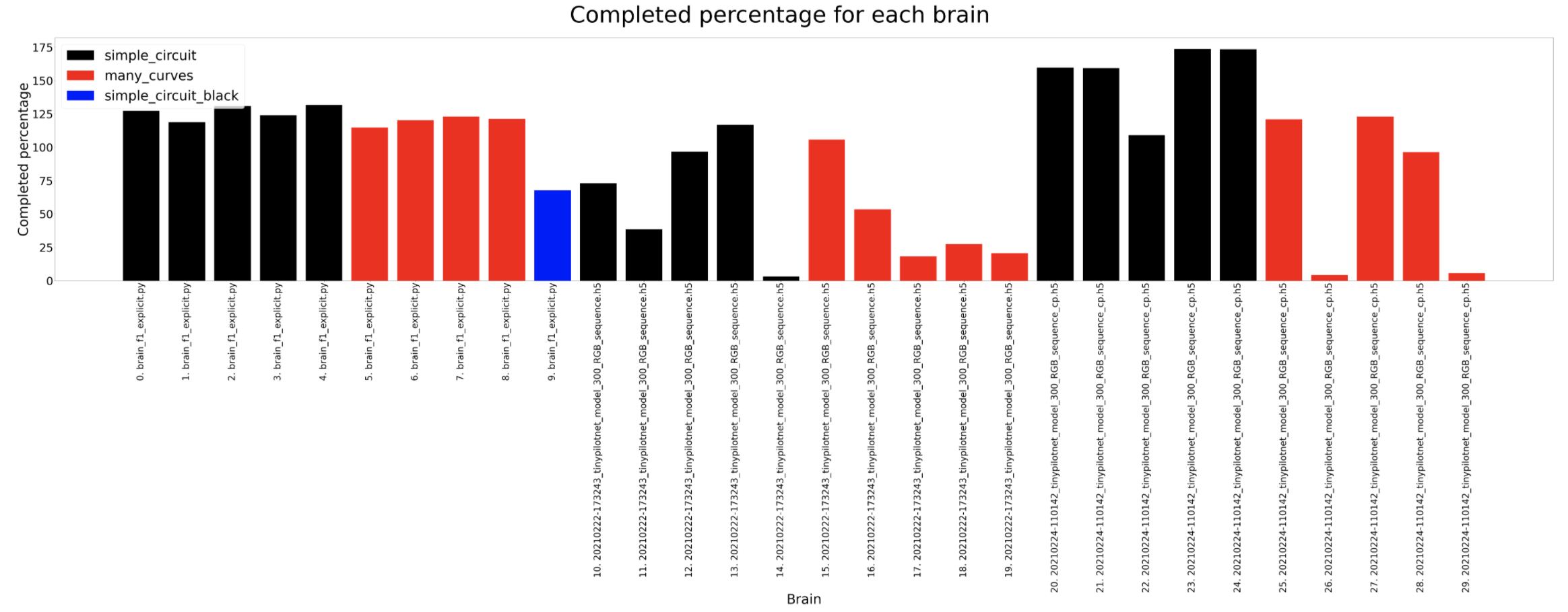
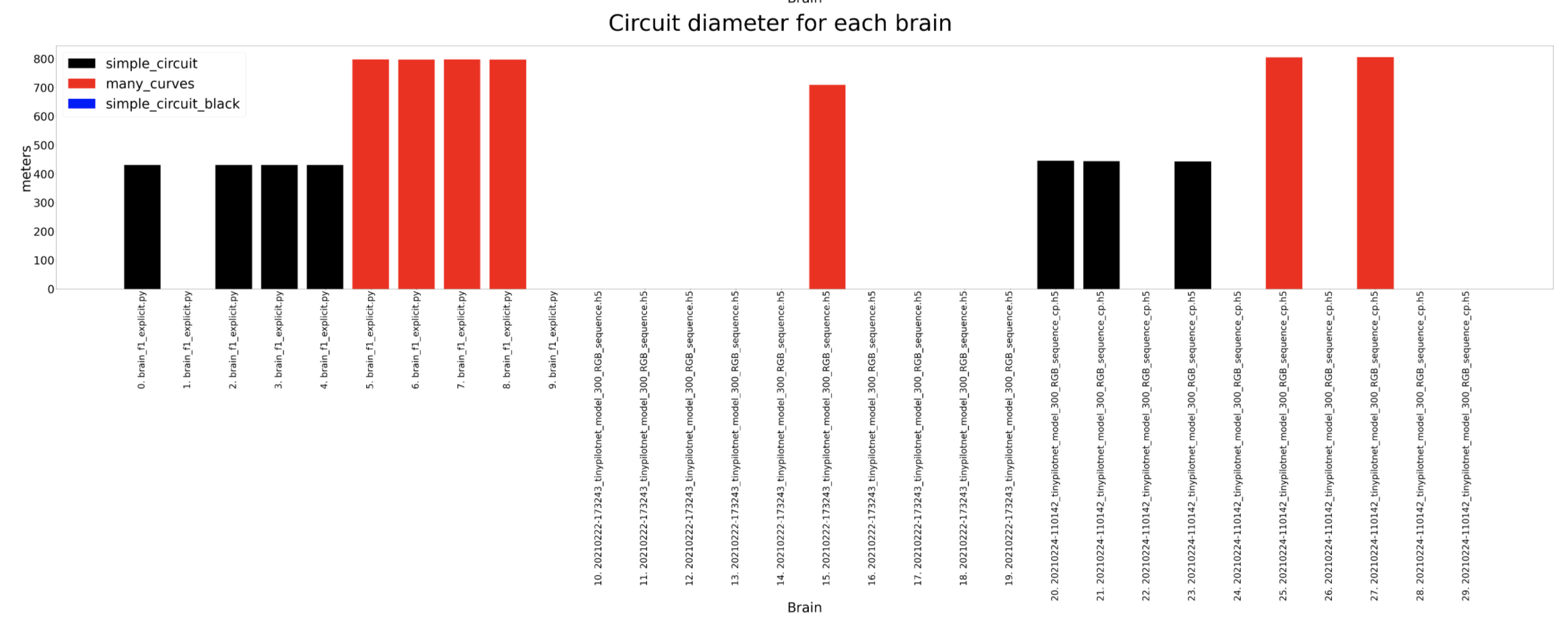
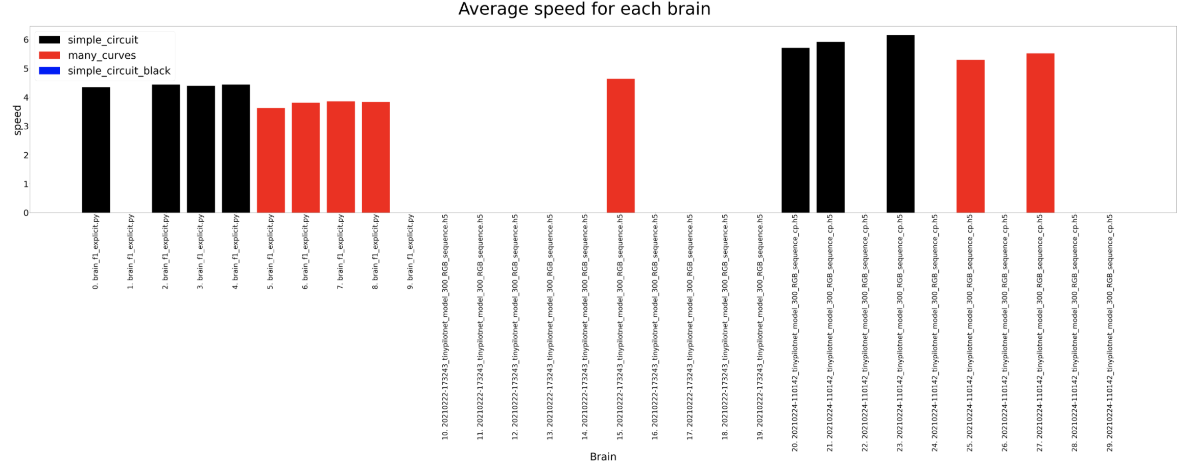
In this section we are going to analyse the results for the different brains in 2 test circuits. For the experiments, each brain is run 5 times on each circuit in order to have reliable data to analyse.

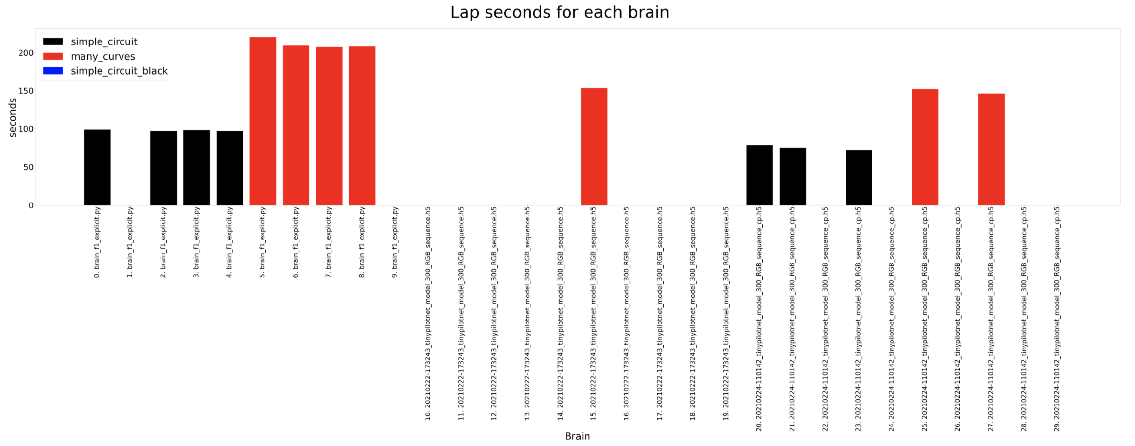
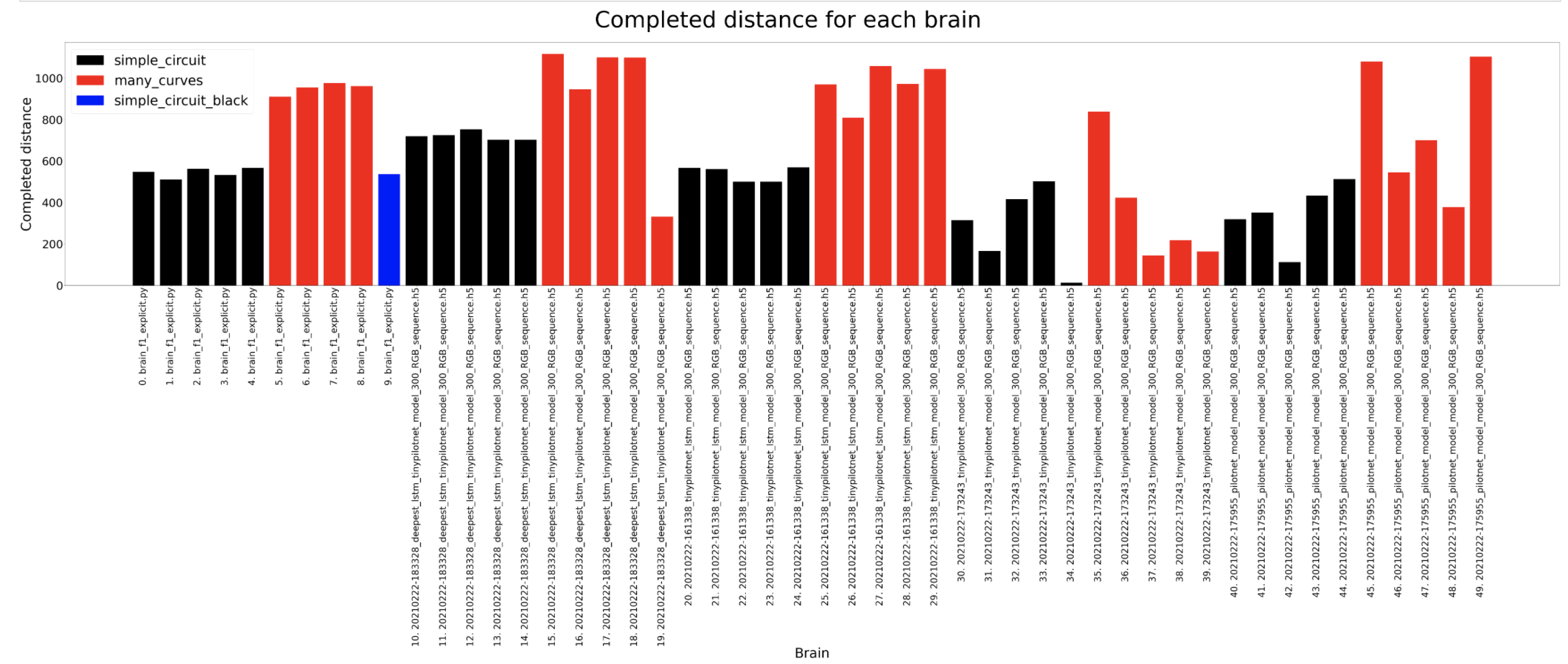
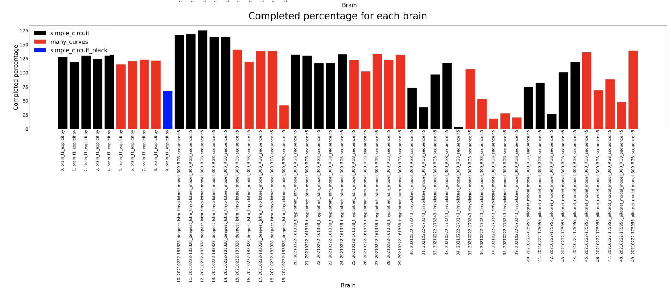
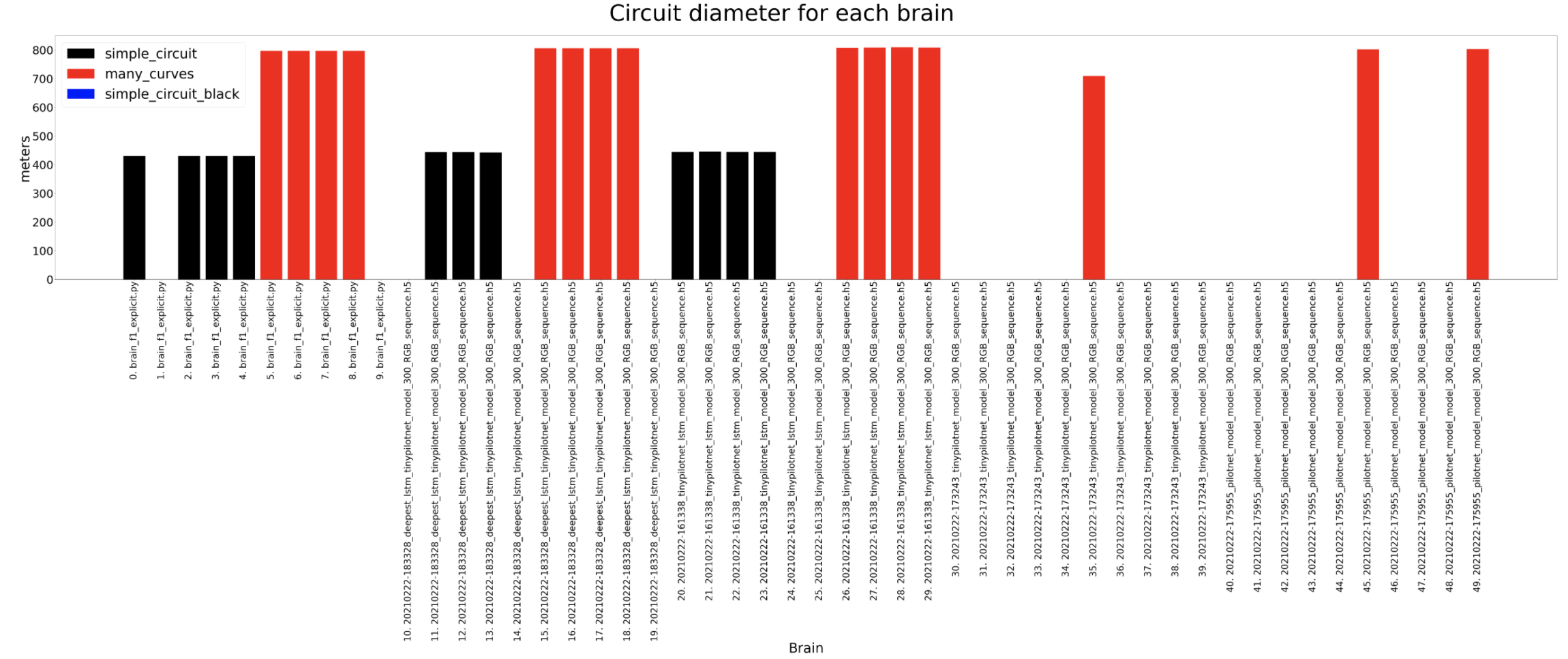
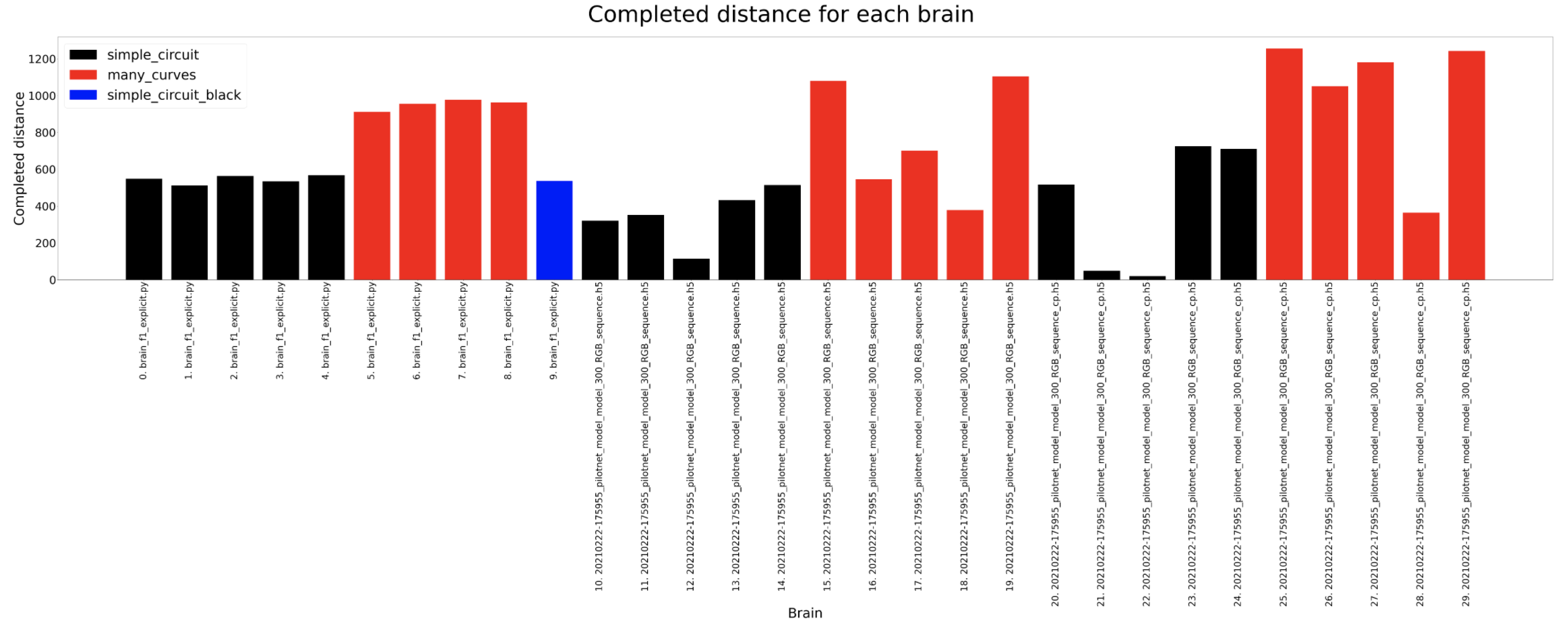
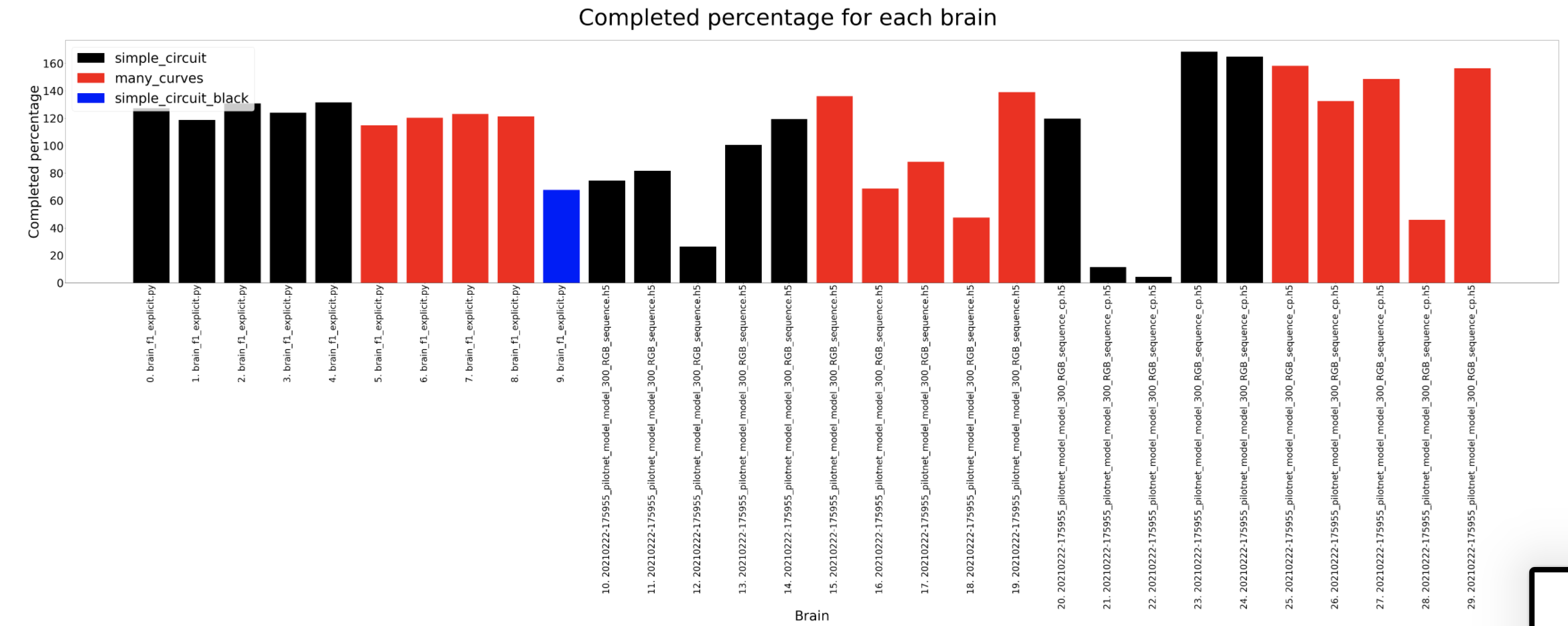
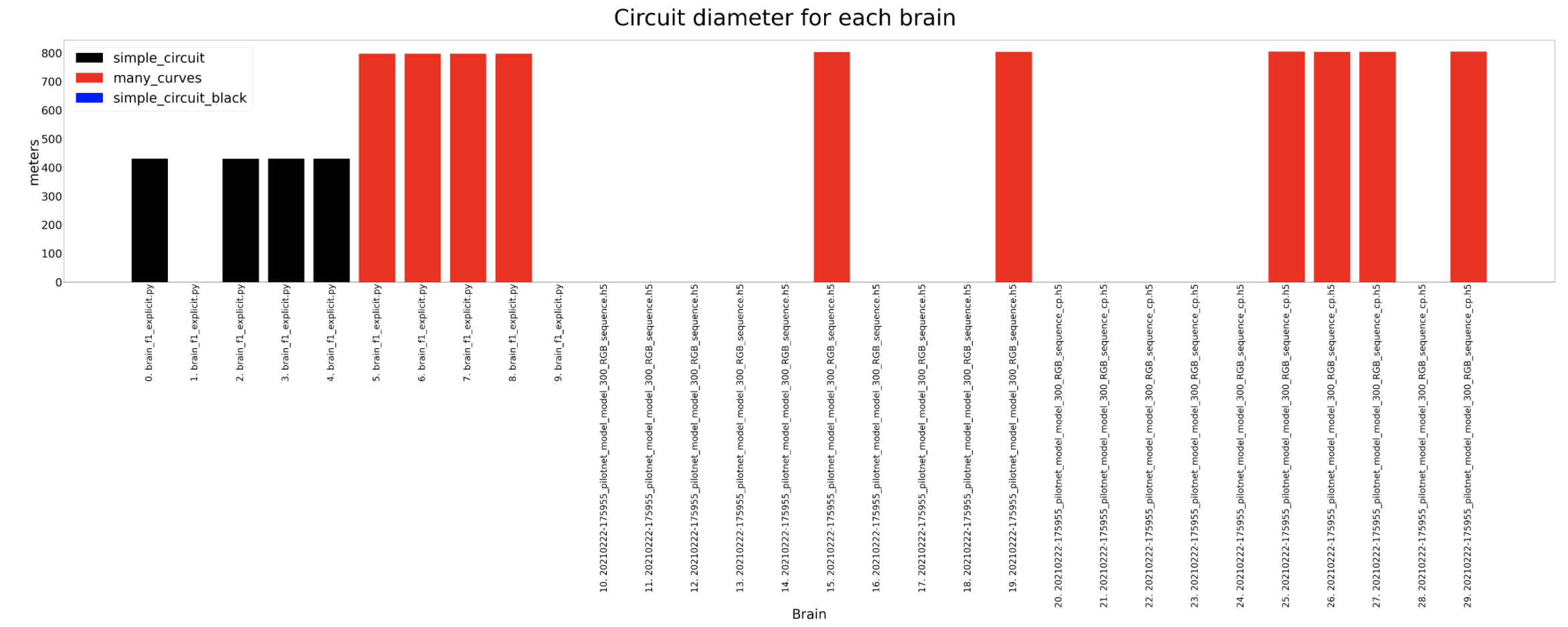
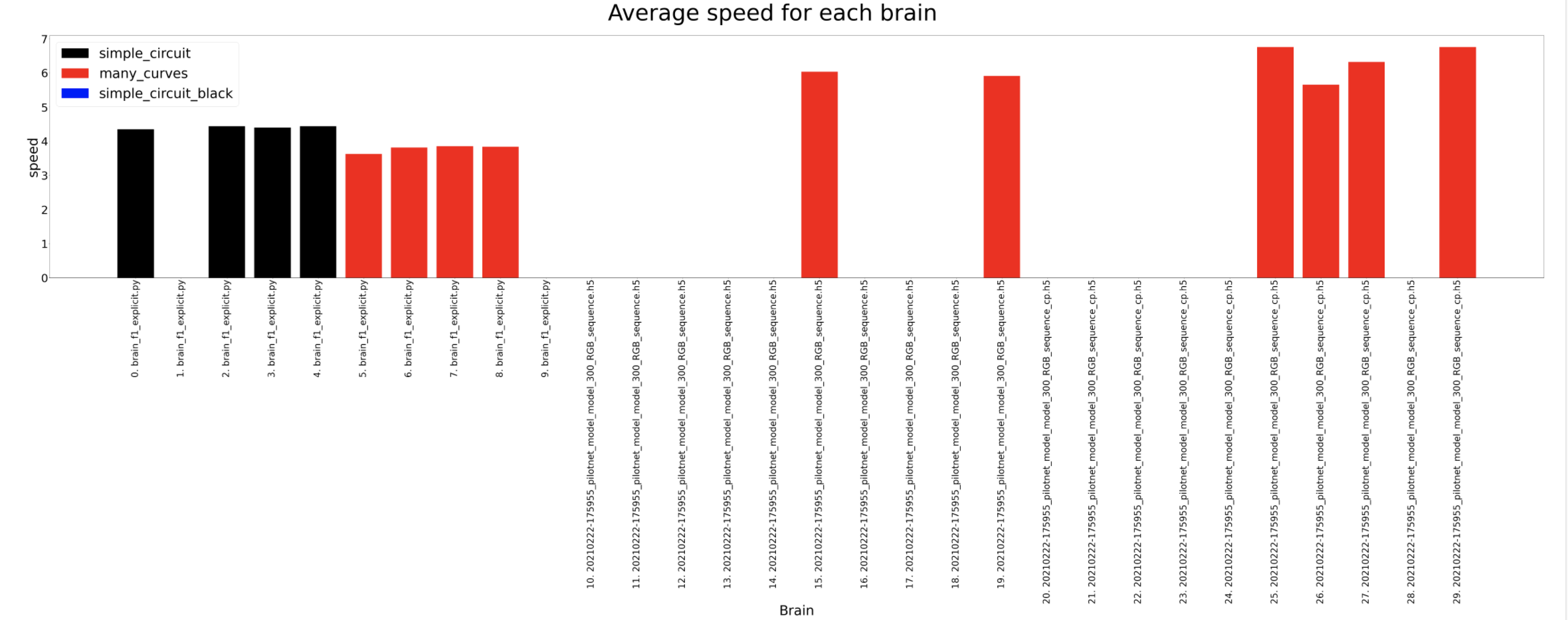
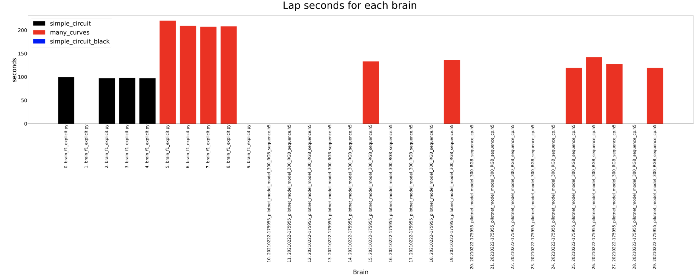
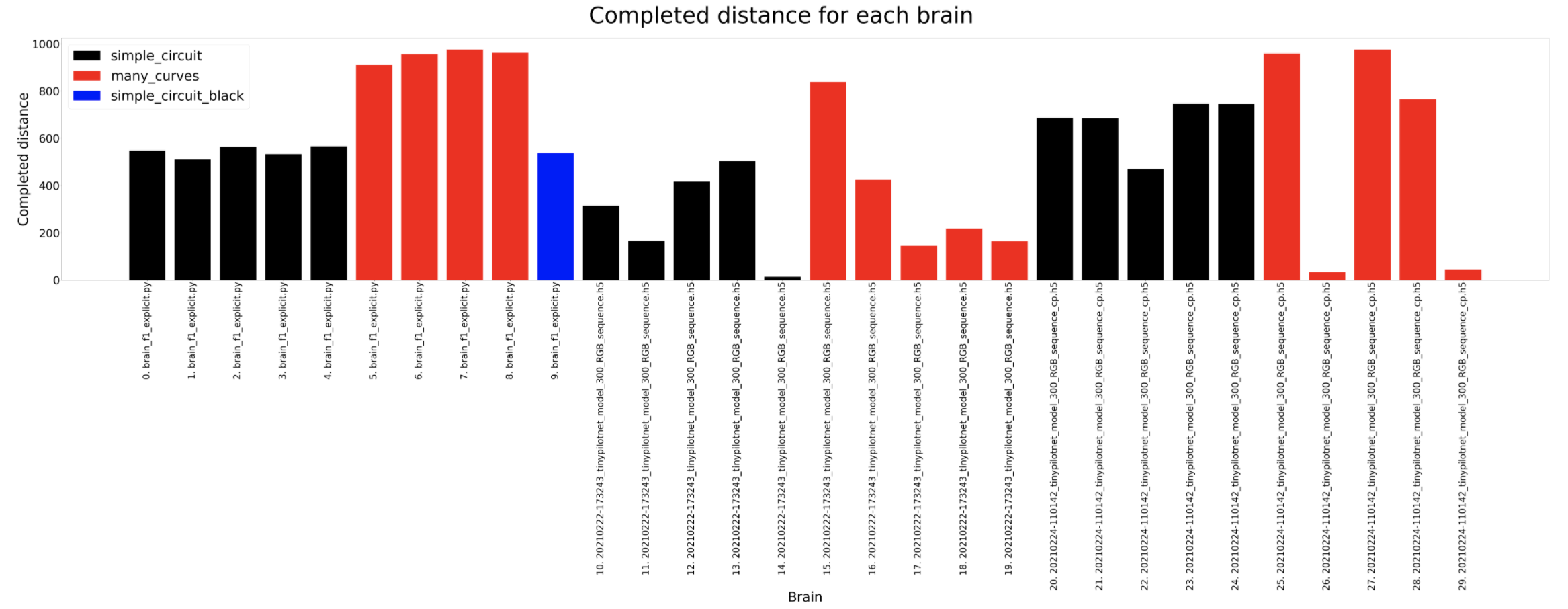
In these experiments the most amount of data is captured so then we can understand deeply what is going on inside the brain. The timeout for each experiment for a certain circuit is always the same, 120 seconds for the simple circuit and 180 for the many curves. For the completed distance, we can detect that the many curves circuit is longer and that the deepest lstm network usually completes the longer distance where as the tinypilotnet is the one performing worse. The completed percentage should look quite similar to the previous result and that is what actually happens. In the circuit diameter we can detect some weird scenarios. This columns show the circuit diameters only for the brains that have completed a lap. As we can see, the first 3 brains are better than the 2 on the left. If we look at the third column from the left hand side, for a tinypilotnet brain the circuit diameter is less than for the rest of the brain for that same circuit (many curves as its red). This means that this experiment has experimented some trouble an its erroneous, so we should not consider the tinypilonet network to have completed any lap at all.

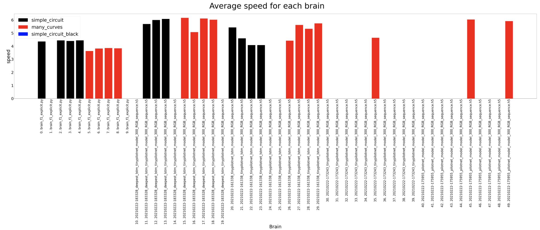
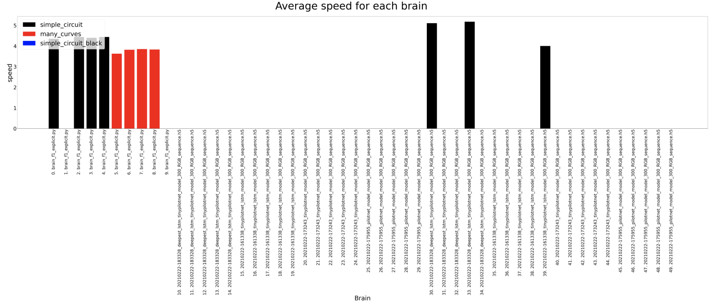
The average speed shows some interesting conclusions. The explicit brain is the one used to generate the dataset and is considered the reference. We expect the brains to be slower than this brain but as we can see, the deepest lstm tinypilonet is always faster.

Click on the images to expand them.

Completed distance

Completed percentage

Circuit diameter

Average speed

Lap seconds

Results in test circuits with modifications

Now that we have covered results for several brains in the 2 circuits available, here we present some modifications to those experiments to test a little bit further the brains. These experiments involve a modification of the simple circuit and a modification on the images input to test the resilience of the networks and understand what they are learning.

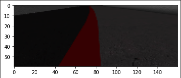
In the first case, the simple circuit walls color are changed to black (in the raw simple circuit they are white). This change is made in order to understand if the walls color has something to do in the behavior of the brains. As we can see in the results (columns in blue), the brains can’t usually complete the circuit due to this condition, even taking into consideration that the images are cropped (see bottom figure).

In the second scenario, the input images color channels are changed from RGB to BGR. In this case, the results show that the networks based on LSTMs are resilient enough to still manage to complete the circuit, whereas the only CNN options have more problems.

Completed distance

Completed percentage

Circuit diameter

Average speed

Lap seconds

Cropped image

Results with PilotNet checkpoint

Checking back the results for PilotNet, we can understand that this brain performance is ok but it sometimes fails to complete the circuit. In this experiment, we explore the performance of PilotNet checkpoint network. This network is just the same as the previous one but on its best point in training, instead of in the 300 epoch. As we can see, its performance is better than for the 300 epoch network. It’s still not good enough when compared to the other networks based on LSTMs but it’s performance is quite good.

Completed distance

Completed percentage

Circuit diameter

Average speed

Lap seconds

Results for TinyPilonet with L2 regularization

In this experiment tinypilonet is retrained with L2 regularization in the Dense layers after the convolutional layers. Trained again for 300 epochs, we obtain a much better network that outperforms the previous Tinypilonet implementation. Once again, we select the checkpoint for the best trained network instead of the network at 300 epochs an the results are as follows, clearly improving the performance.

Completed distance

Completed percentage

Circuit diameter

Average speed

Lap seconds