Included random initial positions and random perturbations to cartpole problem
IMPLEMENTATION
To success with the basic approach (“easy” start position and no perturbations) we implemented double dqn making use of a target neural network that execute the steps and is periodically updated with other neural network that is being trained from the experience. This, together wih the replay buffer was not enough to make it stable:
- The success of the training highly depends on how the training starts. If the neural network starts learning, it will behave well, otherwise, it will not learn nothing from the very beginning.
- After some iterations learning (and most of the time reaching the optimal learning) the performance decrease and the neural network forget to solve the problem. This is a common problem called “catastrophic forgetting”.
So we tried to solve the problems with the following actions:
- Don’t decrease the epsilon (exploration rate) until some configurable iterations. In that way we ensure our agent starts exploring the world without taking wrong learned decissions until we feel it explored enough.
- We blocked some entries in the replay buffer so we ensure that when the agent learns to solve the problem, we still have some unsuccessful scenarios to train the neural network (and it may not forget the learned policies)
None of them worked as expected, so we had to:
- Save the model periodically upon configuration so we got some brain if the neural network forgets at some point.
- We set by configuration a parameter “objective_reward” to stop learning when the goal is already reached
- Tune the hyperparameters so we start taking optimal actions not too late and we learn at a velocity and a duration in which our problem solution is nearly always learned.
Once we got the most stable solution we could reach, we started making the problem harder with the two following configuration parameters:
- random_start_level: it indicates how wide is the spectrum of possible initial states which the agent must recover from
- random_perturbations_level: it indicates how often a random perturbation is provoked to the pole.
- perturbation_intensity: it indicates how intense is the provoked perturbation to the pole. It must be an Integer.
After tons of trials, the agent could not learn when we change the problem to a more difficult one. However, after learning in the simple scenario, the pole was able to recover from a wide spectrum of situations as we will see in the following section. For more info ou can check the simulated anealing algorithm
DEMO
That said, our goal is to prove that we are able to train an agent that can recover the pole even trying to boycott it. All the following scenarios were run with the agent shown in the following video (same than previous post), that was trained with the following hyperparameters:
- gamma: 0.95
- epsilon_discount: 0.9998
- batch_size: 256
EXPERIMENTS
WITH RANDOM INITIAL STATES
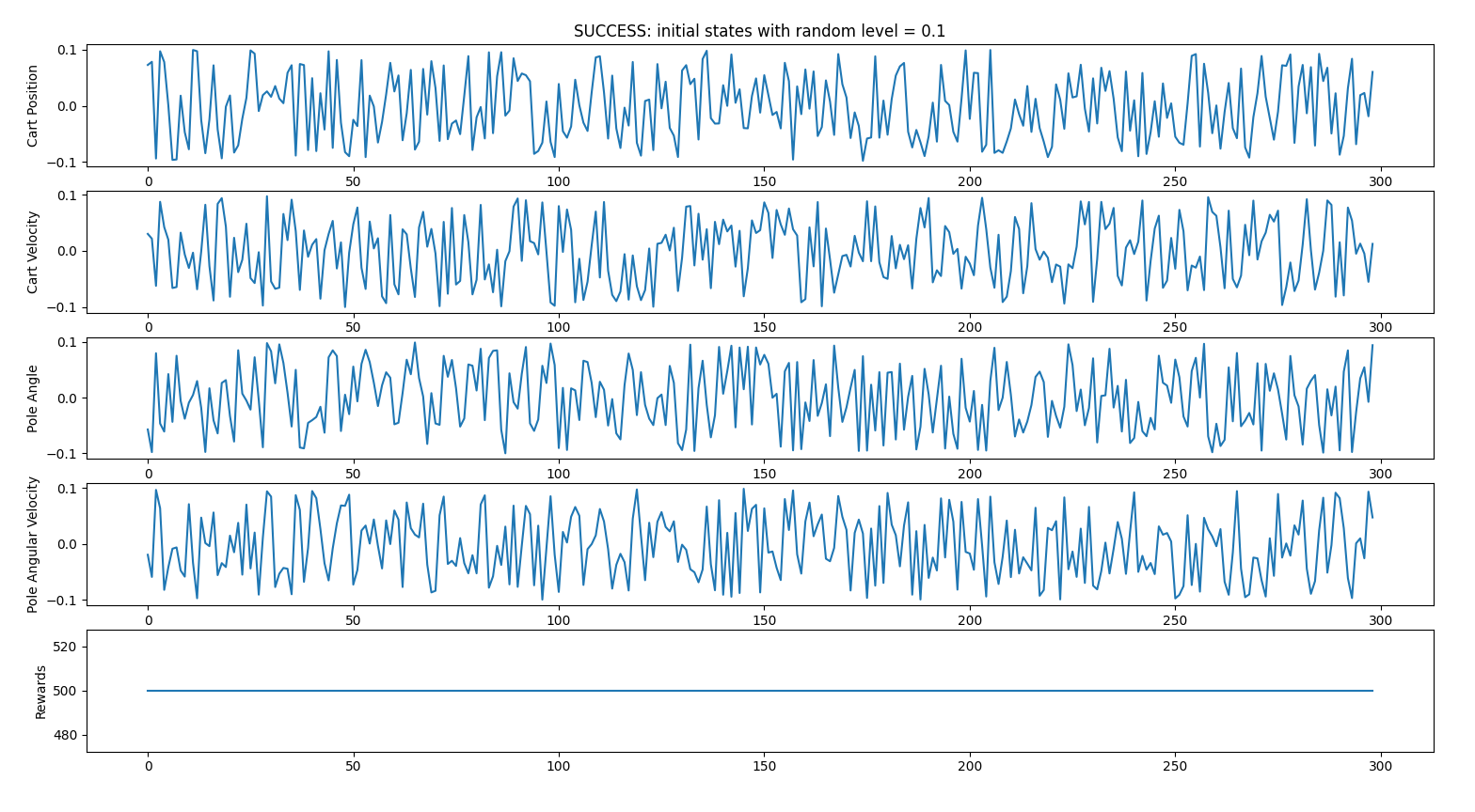
RANDOM INITIAL STATES CASE 1
- random_start_level = 0.1 (all initial states attributes will be between -0.1 and 0.1)
0 failed iterations vs 300 succeeded iterations => 100% success
Successful iterations
Failed iterations
No failures (i.e every iteration reached 500 steps)
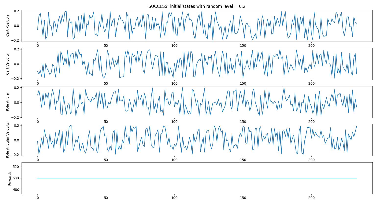
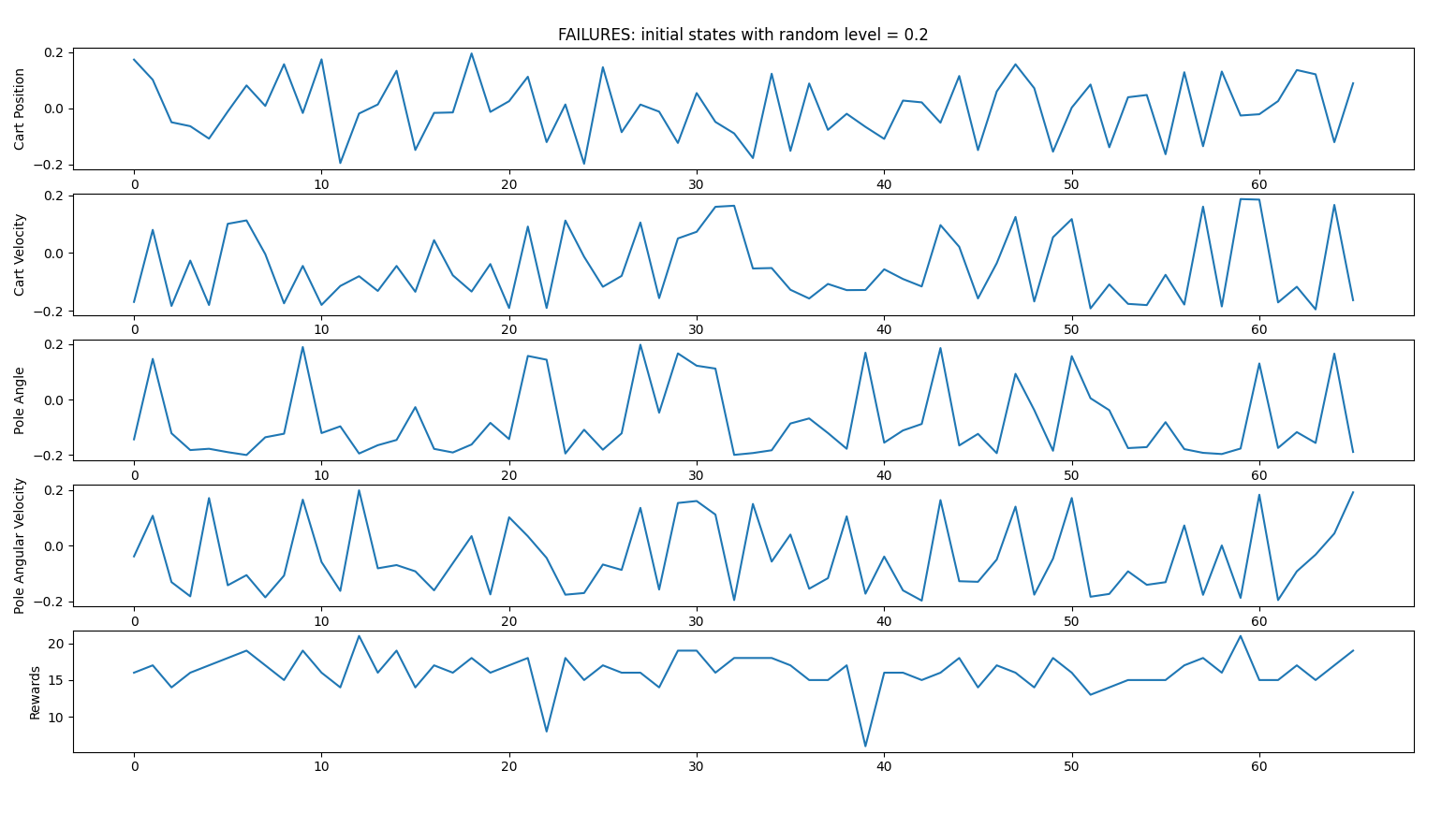
RANDOM INITIAL STATES CASE 2
- random_start_level = 0.2 (all initial states attributes will be between -0.2 and 0.2)
66 failed iterations vs 234 succeeded iterations => 88% success
Successful iterations
Failed iterations
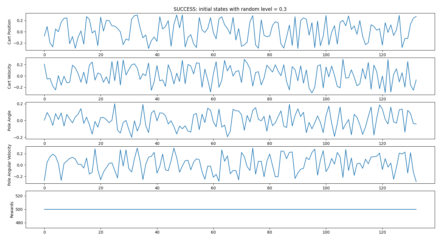
RANDOM INITIAL STATES CASE 3
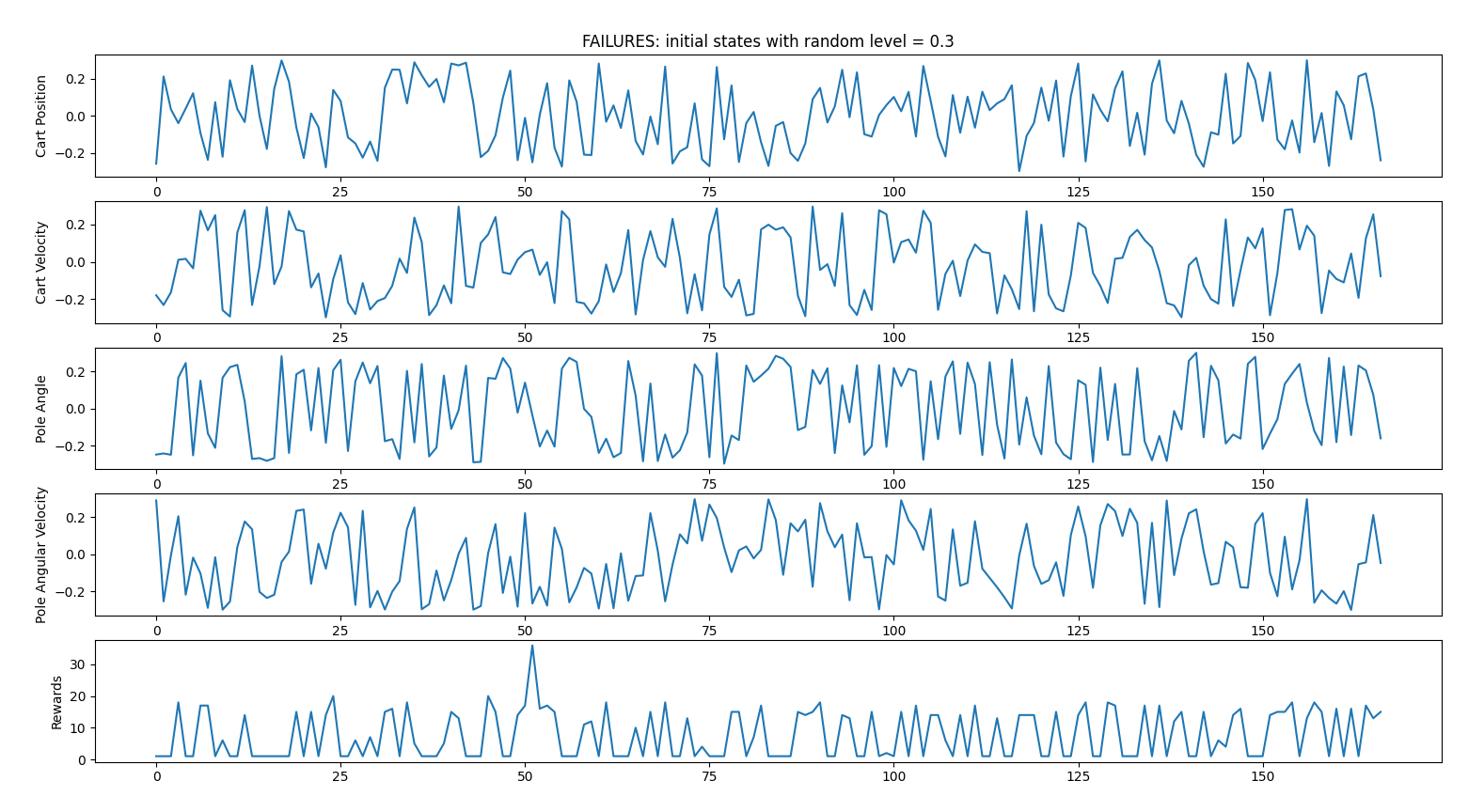
- random_start_level = 0.3 (all initial states attributes will be between -0.3 and 0.3)
123 failed iterations vs 177 succeeded iterations => 59% success
Successful iterations
Failed iterations
RANDOM INITIAL STATES CASE 4
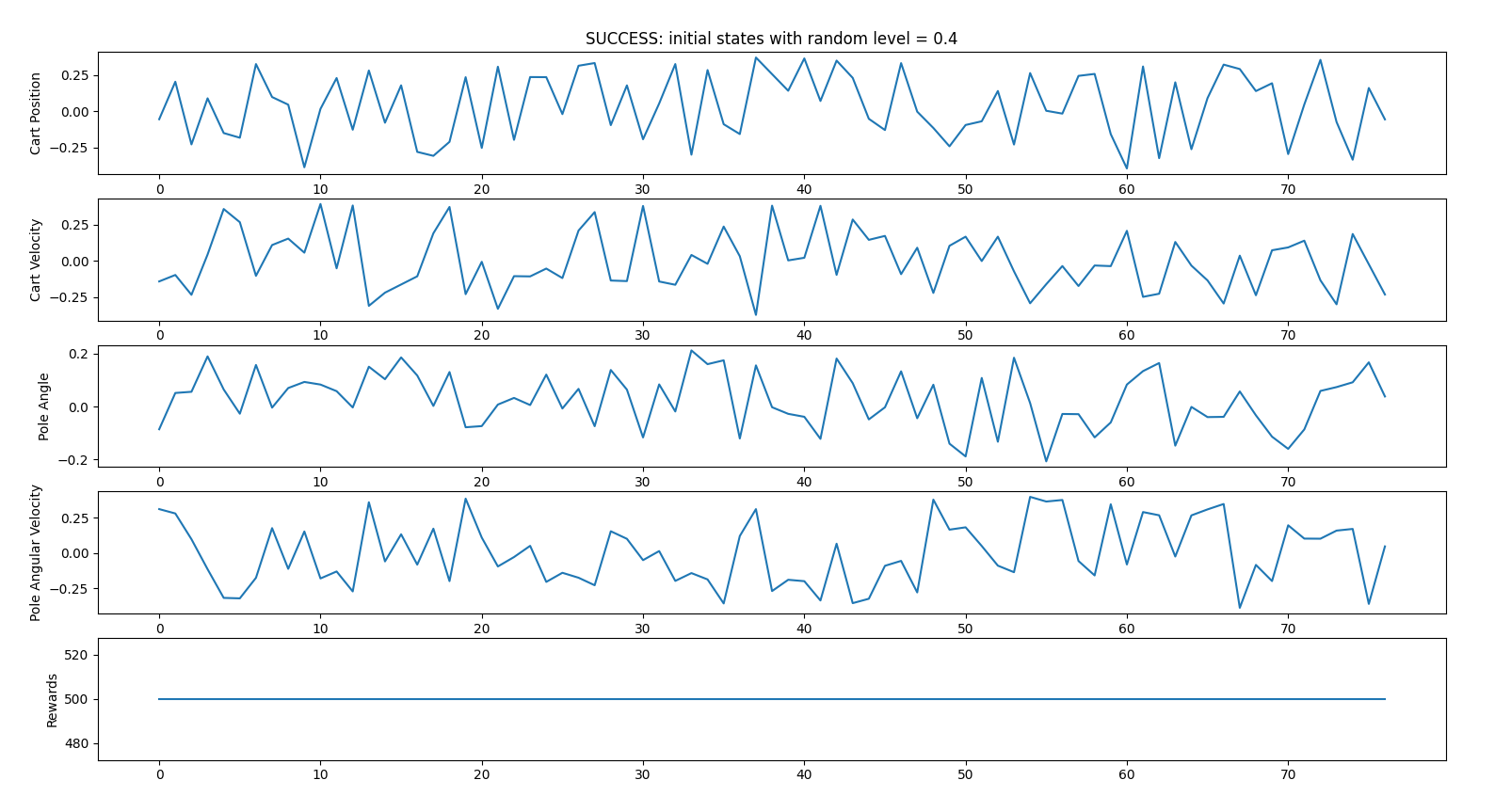
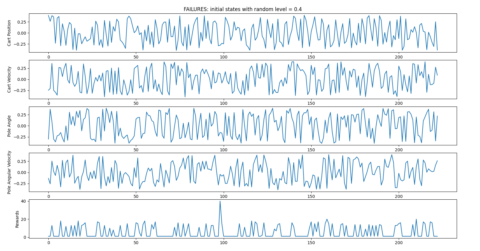
- random_start_level = 0.4 (all initial states attributes will be between -0.4 and 0.4)
222 failed iterations vs 78 succeeded iterations => 26% success
Successful iterations
Failed iterations
WITH RANDOM PERTURBATIONS
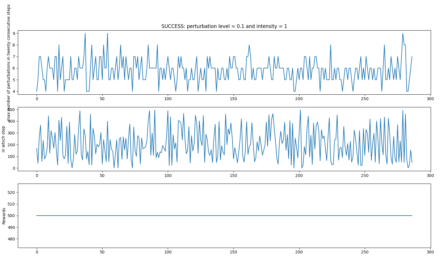
RANDOM PERTURBATIONS CASE 1
- random_perturbations_level = 0.1 (perturbation in 10% of control iterations)
- perturbation_intensity = 1

Successful iterations
Failed iterations

Average: 479.43333333333334 time spent 0:25:14.425255
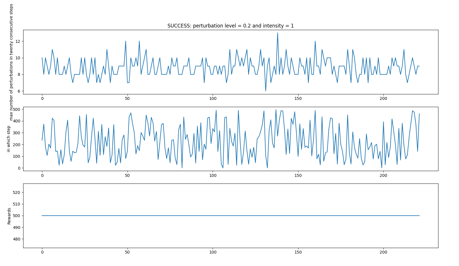
RANDOM PERTURBATIONS CASE 2
- random_perturbations_level = 0.2 (perturbation in 20% of control iterations)
- perturbation_intensity = 1
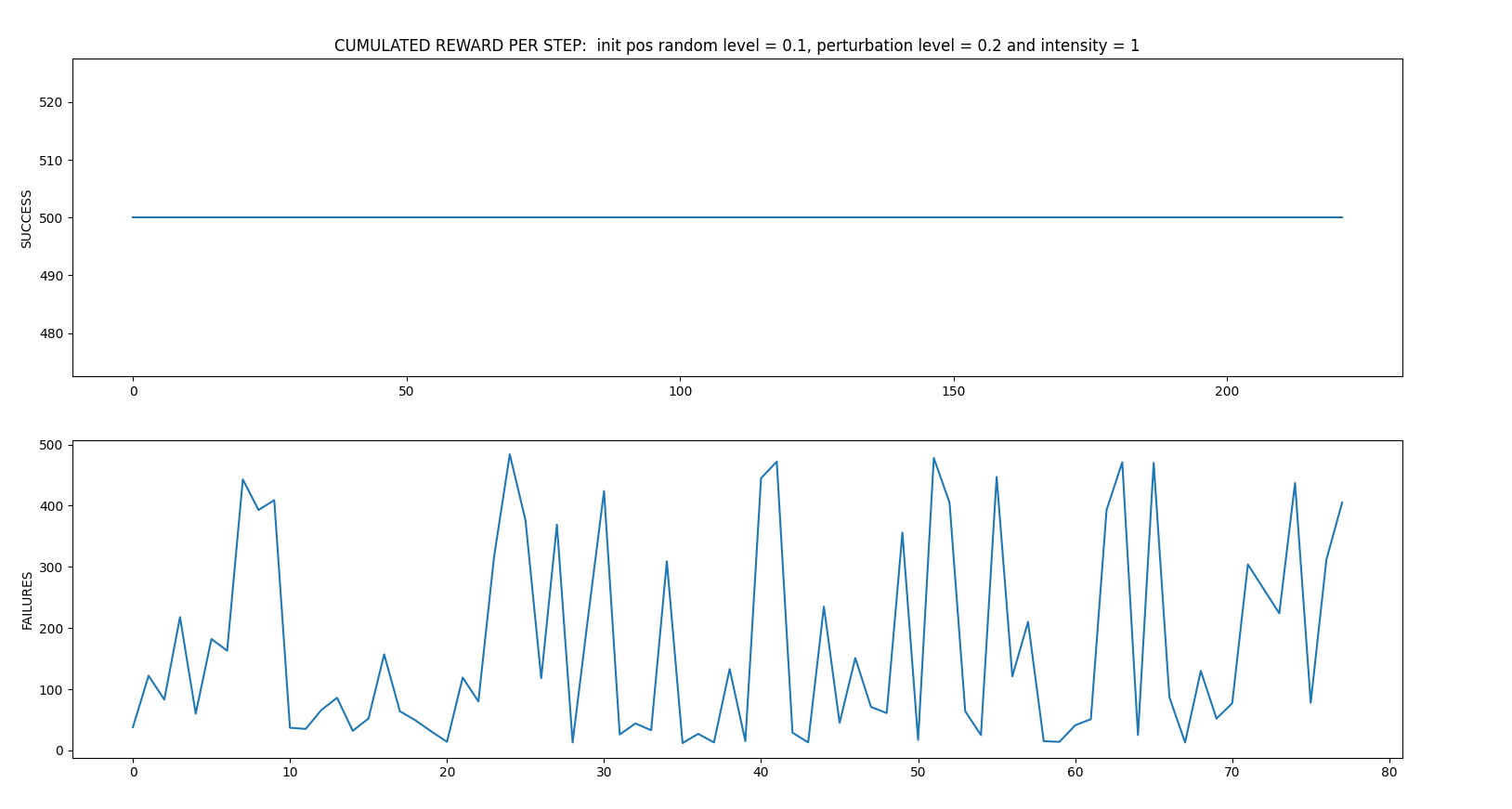
Successful iterations
Failed iterations
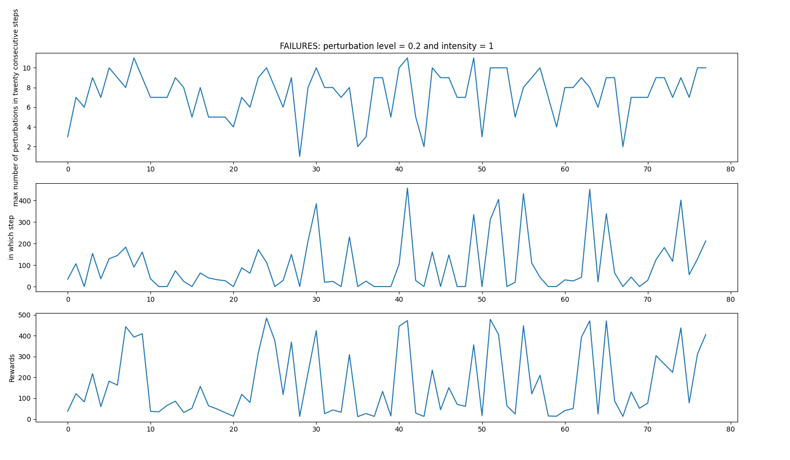
Average: 414.5833333333333 time spent 0:21:52.976723
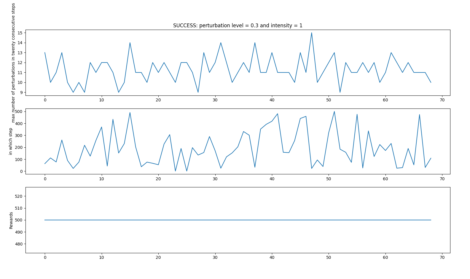
RANDOM PERTURBATIONS CASE 3
- random_perturbations_level = 0.3 (perturbation in 30% of control iterations)
- perturbation_intensity = 1
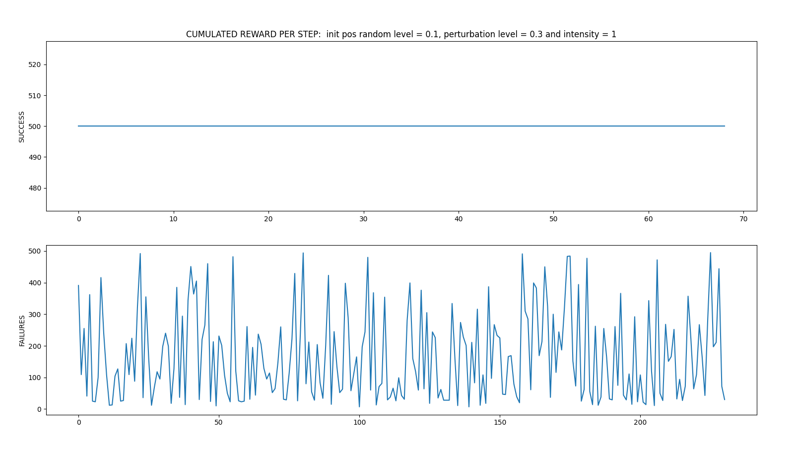
Successful iterations
Failed iterations
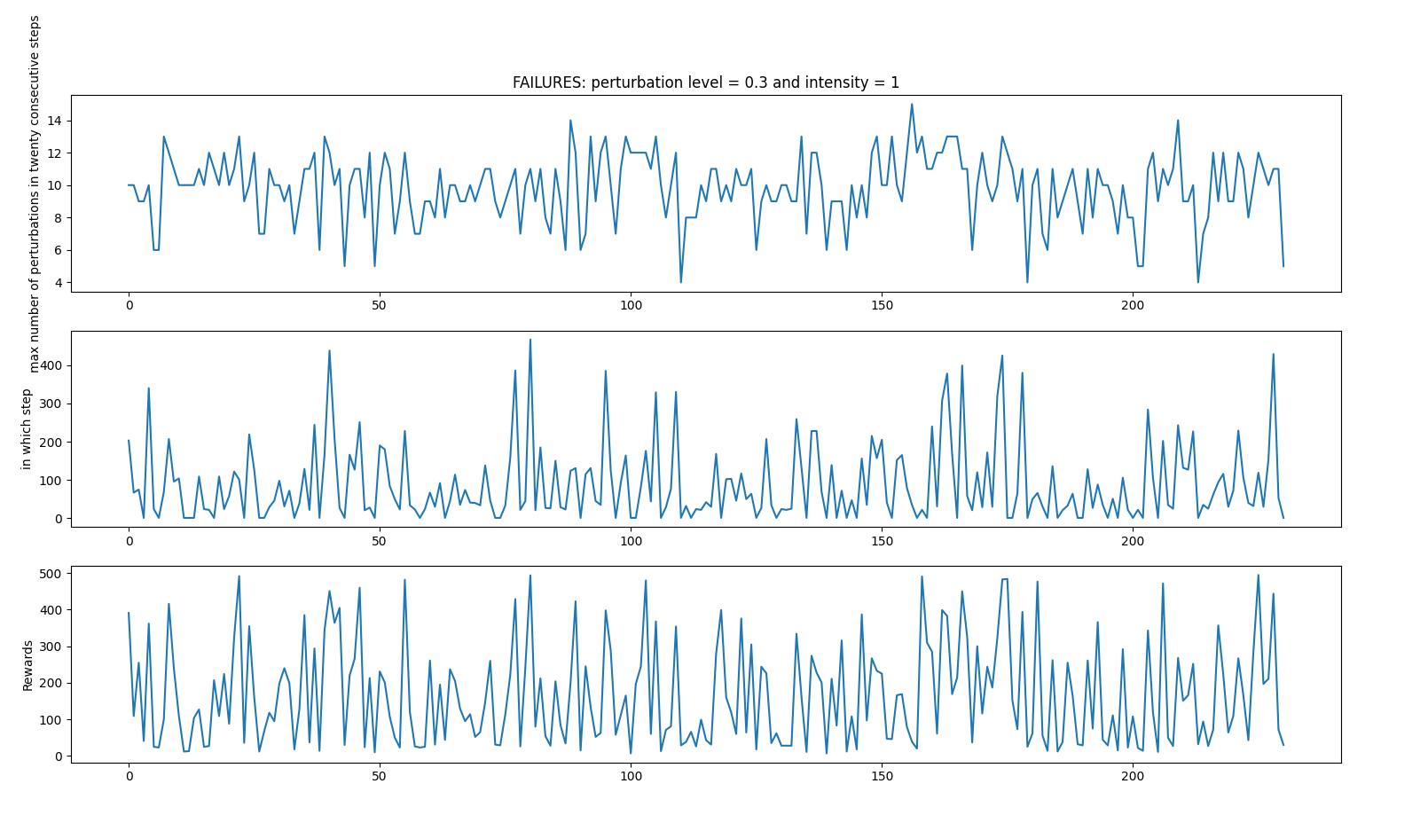
Average: 243.72 time spent 0:12:54.998979
WITH DIFFERENT PERTURBATIONS INTENSITIES
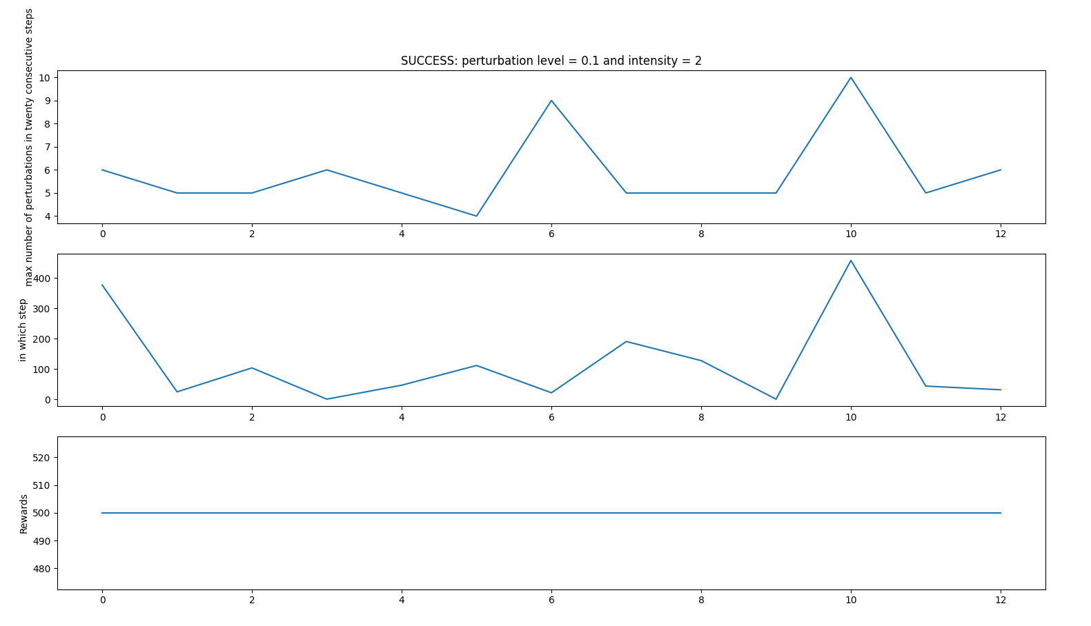
PERTURBATIONS INTENSITIES CASE 1
- random_perturbations_level = 0.1 (perturbation in 10% of control iterations)
- perturbation_intensity = 2 (2 times more intense than in previous experiments)
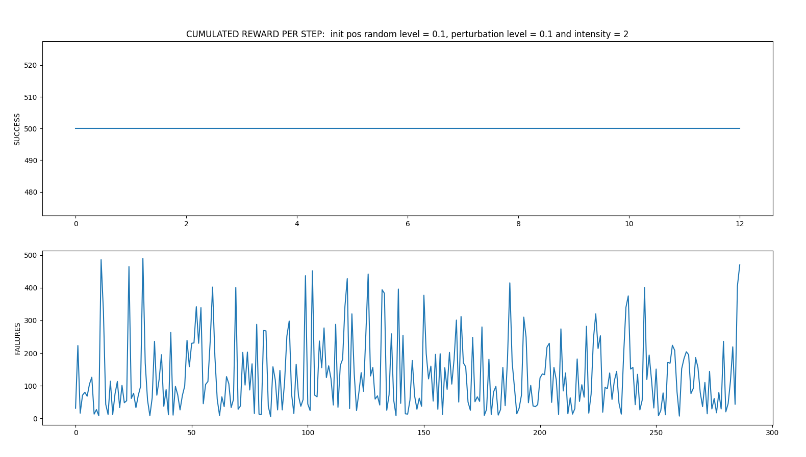
Successful iterations
Failed iterations
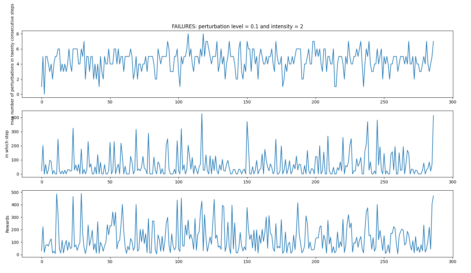
Average: 147.16666666666666 time spent 0:07:44.651692
PERTURBATIONS INTENSITIES CASE 2
- random_perturbations_level = 0.1 (perturbation in 10% of control iterations)
- perturbation_intensity = 3 (3 times more intense than in previous experiments)
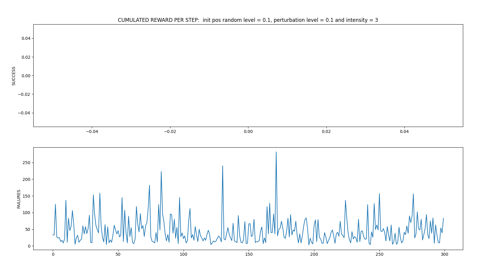
Successful iterations
No success (i.e iteration reached 500 steps)
Failed iterations
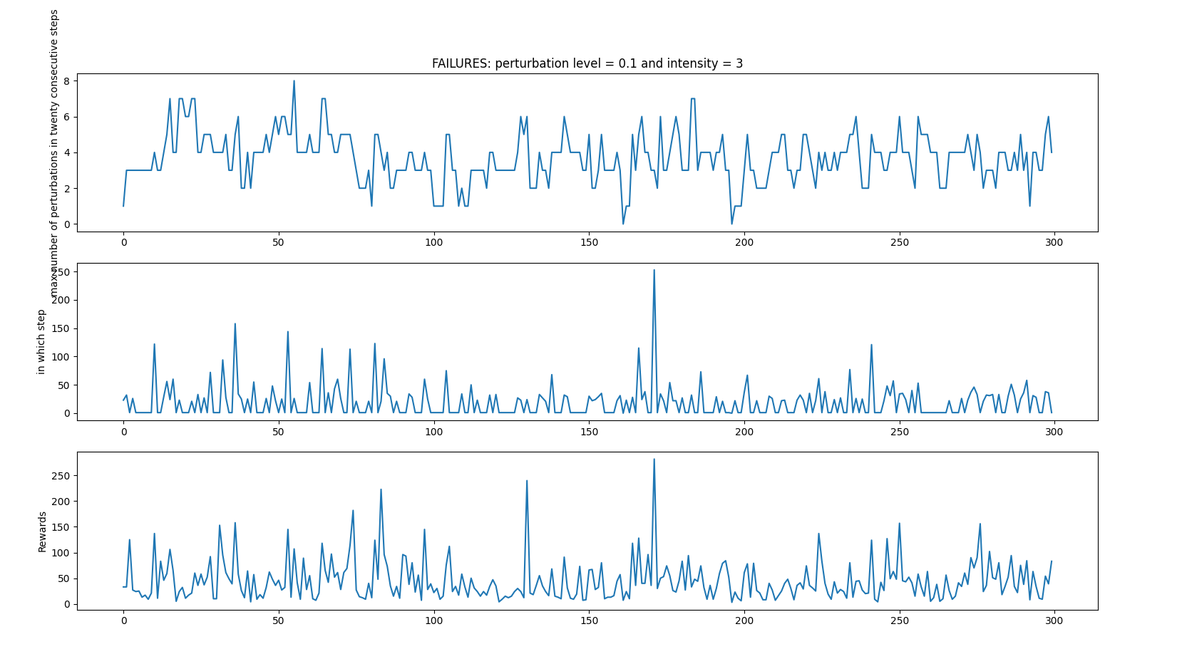
Average: 45.406666666666666 time spent 0:02:24.456620
CONCLUSIONS
- It is important to start from an easy problem when training and then, iteratively train this trained brain with different more complex situations
- If you keep training too much time when uising neural networks, you may run into the catastrophic forgetting problem. Save your model periodically and make sure you train with the correct hyperparameters (mainly learning rate and replay buffer size) and the correct duration
- The dqn algorithm trains better than qlearning, and it is able to recover from quite intense perturbations and random initial positions.
The thresholds from with the agent is able to recover in terms of initial position and perturbations is the following:
- Initial state attributes (cart position, pole angle, cart velocity and pole velocity) set between -0.2 and 0.2 except when:
- The pole angular velocity and the cart velocity are set close to the opposite boundary (e.g cart velocity=-0.18 and pole angular velocity=0.19)
- The pole angular velocity and pole position are set close to the same boundary (e.g pole position = 0.19 and pole angular velocity=0.17))
- The pole is able to keep up when
- frequency of perturbations is in 20% of control iterations with low intense (and not bad performance also with 30%)
- being the frequency of 10% of control iterations, the intensity is two times bigger than the agent actions
- Initial state attributes (cart position, pole angle, cart velocity and pole velocity) set between -0.2 and 0.2 except when: