Gazebo F1 Follow line all algorithms comparison
Configuration
QLEARNING
Hyperparameters
alpha: 0.2
epsilon: 0.95
epsilon_min: 0.05
gamma: 0.9
States
1 input indicating how close is the pixel 10 (starting from the lower part of the image) to he center of the image
Actions
3 possible actions
0: [ 6, 0 ]
1: [ 2, 1 ]
2: [ 2, -1 ]
Reward function
Let ( \text{center} ) represent a value. The reward is computed based on the following conditions:
- If ( \text{center} > 0.9 ):
- ( \text{reward} = 0 )
- If ( 0 \leq \text{center} \leq 0.2 ):
- ( \text{reward} = 100 )
- If ( 0.2 < \text{center} \leq 0.4 ):
- ( \text{reward} = 50 )
- Otherwise:
- ( \text{reward} = 10 )
DQN
Hyperparameters
alpha: 0.9
gamma: 0.9
epsilon: 0.2
epsilon_discount: 0.99965
epsilon_min: 0.03
replay_memory_size: 50_000
update_target_every: 5
batch_size: 64
States
10 input indicating how close the following pixels are (starting from the lower part of the image) to he center of the image
[3, 15, 30, 45, 50, 70, 100, 120, 150, 190]
Actions
9 possible actions
0: [7, 0]
1: [4, 1,5]
2: [4, -1,5]
3: [3, 1]
4: [3, -1]
5: [2, 1]
6: [2, -1]
7: [1, 0.5]
8: [1, -0.5]
Reward function
Let (P_1), (P_2), (P_3) be proximity rewards at different positions, (v) be linear velocity, (w) be angular velocity, and (R) be the overall reward.
- Compute Proximity Reward:
- P1,done1=reward_proximity(Pstate1)
- P2,done2=reward_proximity(Pstate2)
- P3,done3=reward_proximity(Pstate3)
- Average proximity reward: P=P1+P2+P3/3
where reward_proximity:(1−∣state∣)
- Normalize Linear Velocity:
- vnorm=normalize_range(v,min_linear_velocity,max_linear_velocity)
- Compute Velocity Reward:
- vreward=vnorm⋅P
- Combine Proximity and Velocity Rewards:
- β=beta_1
- R=β⋅P+(1−β)⋅vreward
- Penalize Angular Velocity (prevent zig-zag behavior):
- wpunish=normalize_range(∣w∣,0,max_angular_velocity)⋅punish_zig_zag_value
- R=R−(R⋅wpunish)
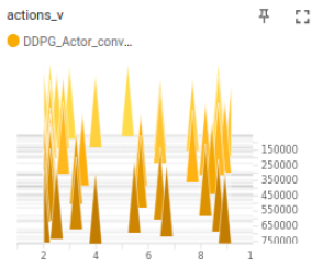
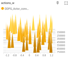
DDPG
Hyperparameters
steps_to_decrease: 20000
decrease_substraction: 0.01
decrease_min: 0.03
reward_params:
  punish_zig_zag_value: 1
  punish_ineffective_vel: 0
  beta_1: 0.7
gamma: 0.9
tau: 0.01
std_dev: 0.2
replay_memory_size: 50_000
critic_lr: 0.003
actor_lr: 0.002
buffer_capacity: 100_000
batch_size: 256
States
Same than in DQN algorithm
Actions
v and w continuous within following ranges:
v: [1, 10]
w: [-2, 2]
Reward function
Same than in DQN algorithm
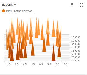
PPO
Hyperparameters
steps_to_decrease: 20000
decrease_substraction: 0.01
decrease_min: 0.03
reward_params:
  punish_zig_zag_value: 1
  punish_ineffective_vel: 0
  beta_1: 0.5
gamma: 0.9
epsilon: 0.1
std_dev: 0.2
episodes_update: 1_000
replay_memory_size: 50_000
critic_lr: 0.003
actor_lr: 0.002
States
Same than in DQN algorithm
Actions
v and w continuous within following ranges:
v: [1, 10]
w: [-1.5, 1.5]
Reward function
Same than in DQN algorithm
Training
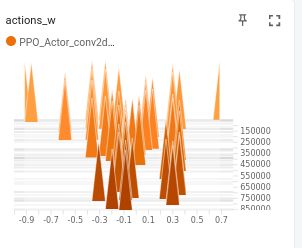
In future implementations, metrics will be recorded and stored in files while launched so they can be graphed afterwards in the same plot. In this experiment we used tensorboard.
Note that training convergence times could be reduced using different decreasing factors or learning rates.
QLEARN
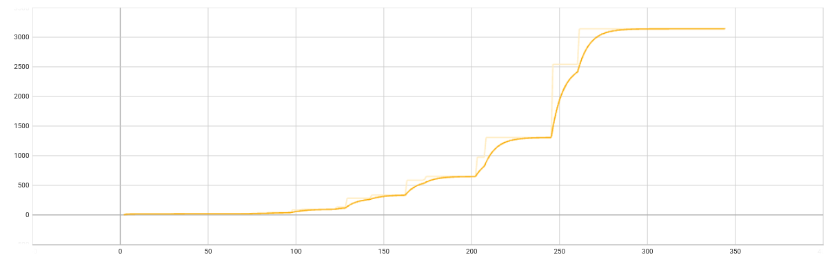
convergence_epoch = 4.723 best_step = 15.001 convergence_epoch_training_time = 0:34:09
DQN
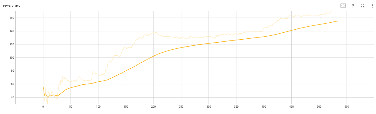
convergence_epoch = 802.302 convergence_epoch_training_time = 22:34:44
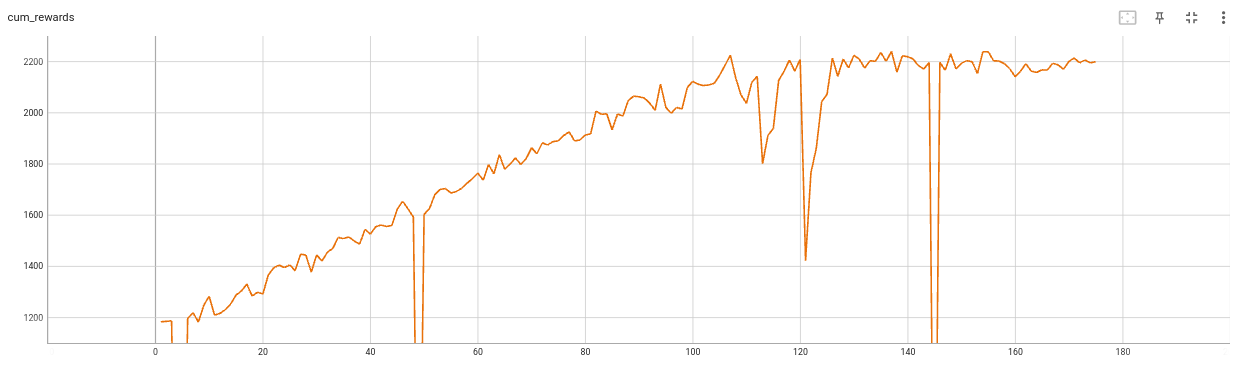
DDPG
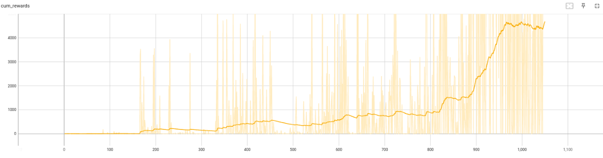
convergence_epoch = 980.020 convergence_epoch_training_time = 56:11:19
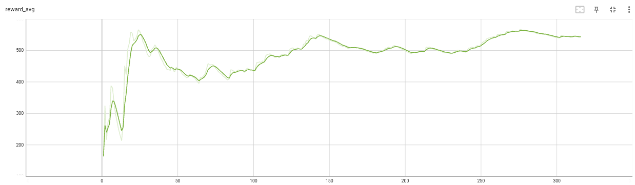
PPO
convergence_epoch = 180.437 convergence_epoch_training_time = 36:11:59
Inference
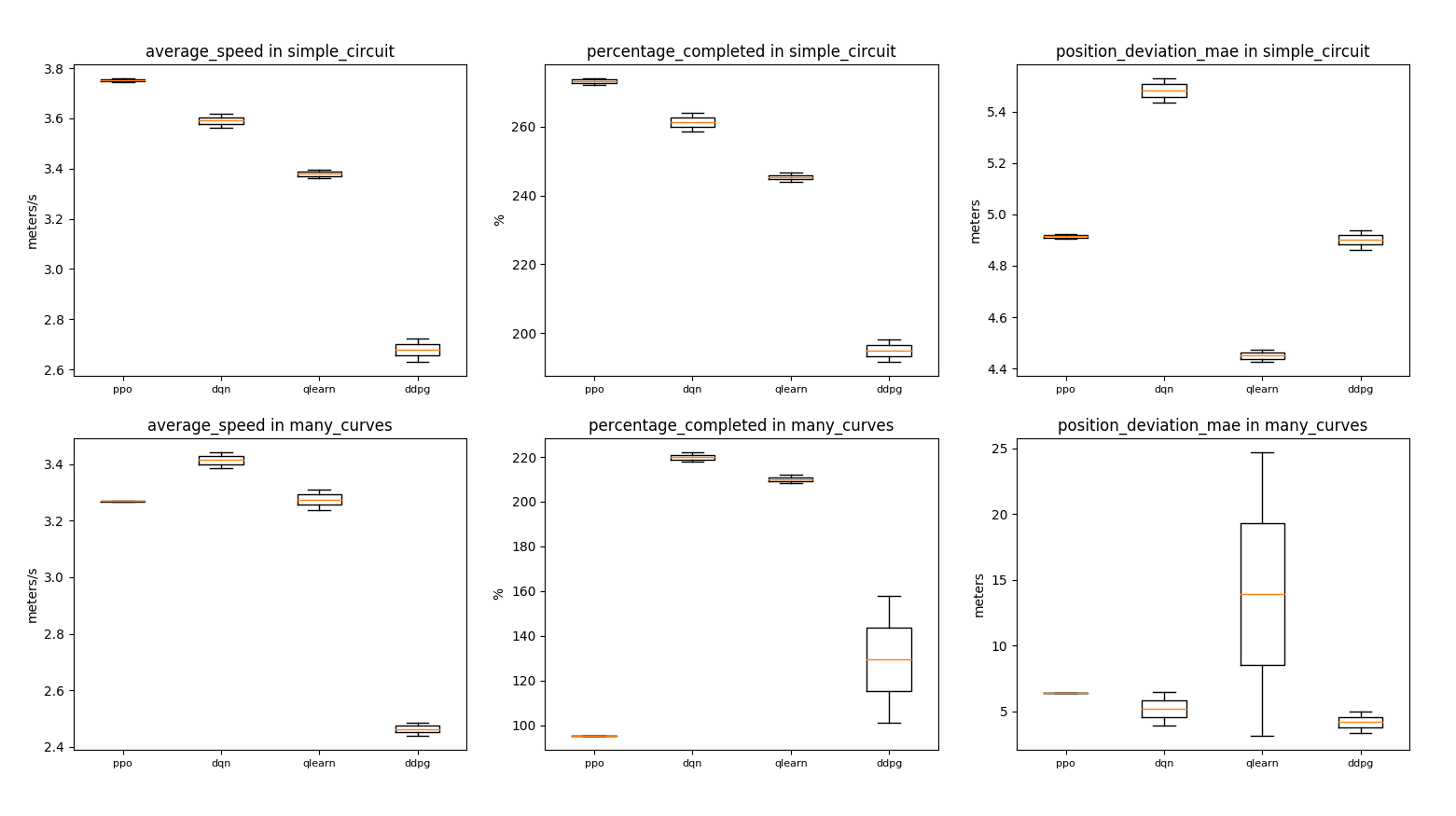
The four best agents were tested on simple circuit where they were trained and on many courves to test generalization.
The 3 metrics measured are speed, circuit completion percentage and deviation with respect to the line:
DEMO
Conclusions
- Both dqn and qlearning looks good enough for this simple task. However, the difference between their proximity to the line in both circuits illustrates that the chosen discrete actions could be good for one circuit and bad for other, making complex to find a feasible discrete actions set that fit to different scenarios.
- The best agent in simple_circuit is ppo, but it overfitted because it is not able to finish the many_courves circuit. Either using a more aggresive epsilon decay to avoid over training or use regularization techniques should work
- The unstability of ddpg while learning seems to contribute to learn a more conservative driving on courves, which also make it slower but safer when using more complex scenarios
Key lessons
- Discrete actions algorithms may converge faster, but actions must be chosen wisely and their optimization may be tedious or even unfeasible
- It is important to keep track of training and inference frequency so we can train with the same (or lower) frequency than inference
- When using continuous actions, it is important to visualize rewards functions so they are as accurate as possible Otherwise, training will be too slow or even suboptimal
- It is key to properly monitor on real time the state-action-rewards, loss function, average reward over time, epsilon (Tensorboard) fps and received image
- If high speed is needed, we must use farther inputs together with the closest ones which will be used to reward the proximity of the agent to the line (car is not in the horizon, car is in the proximal camera image input)
- Actor learning rate must be slightly below critic learning rate so learning rate can adapt to the actor learnings
- Training and infererence must be totally aligned regarding inputs-outputs and all other neural network hyperparameters
- When building a neural network, start with a small one with not too big learning rates to avoid vanishing gradient and overfitting. Then you can iteratively start making it more complex and abrupt
- QLearning and DQN are fine and converge faster for simpler tasks, but they are unfeasible for real AD where we may need too many degrees of freedom on the actions to be applied
- PPO Vs DDPG
- PPO
- Pros:
- Stability: PPO is known for its stability in training, providing more robust convergence properties compared to DDPG.
- Sample Efficiency: PPO tends to be more sample-efficient than DDPG, requiring fewer samples to achieve comparable or better performance.
- Noisy Environments: PPO can handle noisy environments better due to its policy optimization approach.
- Simultaneous Learning: PPO can update its policy using multiple epochs with the same batch of data, allowing for more effective policy updates.
- Cons:
- Slower Training: PPO often exhibits slower training compared to DDPG, especially in terms of wall-clock time.
- Hyperparameter Sensitivity: Fine-tuning PPO can be challenging due to its sensitivity to hyperparameters.
- Pros:
- DDPG
- Pros:
- Learning from Off-Policy Data: DDPG is an off-policy algorithm, enabling learning from previously collected data.
- Cons:
- Instability: DDPG can be sensitive to hyperparameters and initial conditions, leading to instability during training.
- Exploration Challenges: DDPG might face challenges in exploration, especially in high-dimensional and complex environments.
- Limited to Deterministic Policies: DDPG is designed for deterministic policies, which might be a limitation in scenarios where stochastic policies are more suitable.
- Pros:
- PPO