Perception

Introduction

In this post, we will talking about Perception. Switched from PX4 to Client Airsim to gain control of the drone.

Perception

In the previous post we talked about YOLOP and which model to choose to get the best result. From this neural network, we will keep the detected lines of the lanes of the road and we will perform an unsupervised learning algorithm called clustering (DBSCAN) to choose the group of lines that we are interested in the lane to follow, for more details of this algorithm you can visit the following page DBSCAN.

DBCAN

This algorithm classifies a set of samples into groups (clusters) based on the density of points in the feature space. the density of points in the feature space, which is a way of representing data using different measures or attributes. data using different measures or attributes.

It is used to classify the different lines detected by Yolop-320-320.onnx.

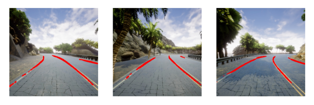
In the following figure you can see the result, contrasting the original image, the result of Yolop-320-320.onnx and DBSCAN.

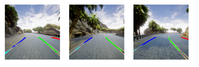
Next, we apply a clustering filtering algorithm to select which cluster groups belong to the lane lines.

Clustering filtering

For the development of the clustering filtering algorithm, we have used a maximised function taking into account the closeness of a central point P and the density of the cluster group points.

Maximized Function Formula

Let ( \text{score_cluster}( \text{cluster}, \text{center} ) ) be a function defined as:

[ \text{score_cluster}(\text{cluster}, \text{center}) = \frac{\text{density}}{\text{proximity}} ]

where:

• ( \text{cluster} = (\text{points_cluster}, \text{centroid}) )
• ( \text{points_cluster} ) is the set of points in the cluster.
• ( \text{centroid} ) is the centroid of the cluster.
• ( \text{center} ) is the reference center.

The proximity (( \text{proximity} )) is calculated as the Euclidean norm between the cluster’s centroid and the reference center:

[ \text{proximity} = | \text{centroid} - \text{center} | ]

The density (( \text{density} )) is defined as the number of points in the cluster:

[ \text{density} = \text{len}(\text{points_cluster}) ]

Therefore, the function ( \text{score_cluster} ) can be expressed as:

[ \text{score_cluster}(\text{cluster}, \text{center}) = \frac{\text{len}(\text{points_cluster})}{| \text{centroid} - \text{center} |} ]

The filtering process can be seen in the following figure:

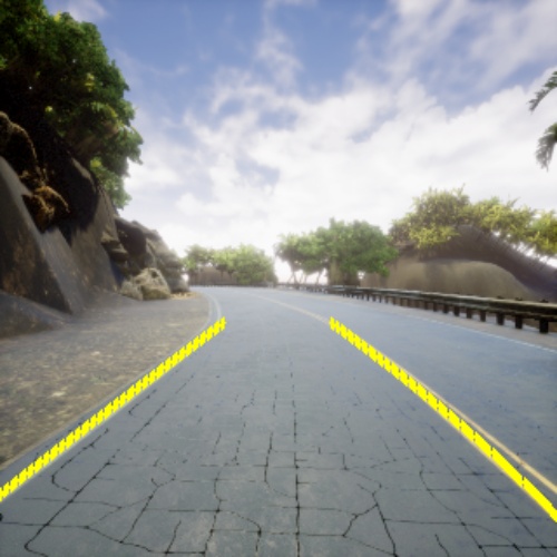
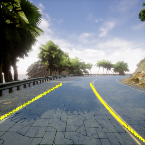
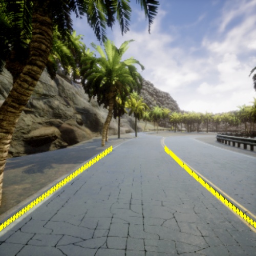
From this algorithm, a reconstruction of the lane lines is performed using quadratic regressions.

Quadratic Regressions

A machine learning technique known as regression is used, which makes it possible to approximate a number N points to a line, curve or other mathematical shape that can be defined by a function. function. As rail lines are rarely completely straight, they are usually curvilinear. In the case of curvilinear lines, a type of quadratic regression is used.

Quadratic regression allows the points in each cluster to be modelled as curves, which is more suitable for capturing the variations of the The quadratic regression technique is more suitable for capturing typical lane variations and curvatures. This technique not only helps to better interpret the shape of the lane, but also makes it easier to navigation of the drone following the trajectory along the lane.

This process is performed twice, a quadratic regression for the group of detected clusters chosen from the right and a quadratic regression for the group of detected clusters chosen from the right. detected clusters chosen from the right and another quadratic regression for the detected cluster group chosen from the left. detected clusters chosen from the left.

Interpolation and calculation of the rail centre of masses

Once the reconstructed lines are obtained, it is necessary to define the rail area within these lines. within these lines.

Therefore, an interpolation is used to traverse and calculate the points that lie within the limits of the regressions.

Finally, the centre of mass of the lane is calculated to obtain the centroid.