Finished Q-Learning 1D
Index
Decreased speed discretisation
The agent accelerates by increasing its speed by 0.1. This implies that if we discretise too sharply the agent may not notice subtle changes in velocity, so the best value for discretisation is 0.1.
Fixed RLidar
In order to use lidar, the agent must be moving, as long as it is static, the rays detect the origin as an obstacle. To solve this problem, noise has been added to the way the origin of the rays is calculated.
1
2
3
4
def add_origin_perturbation(origin, magnitude=0.001):
    """Add noise to origin"""
    perturbation = np.random.uniform(-magnitude, magnitude, size=2)
    return origin + np.array([perturbation[0], perturbation[1], 0])
Example and data analysis
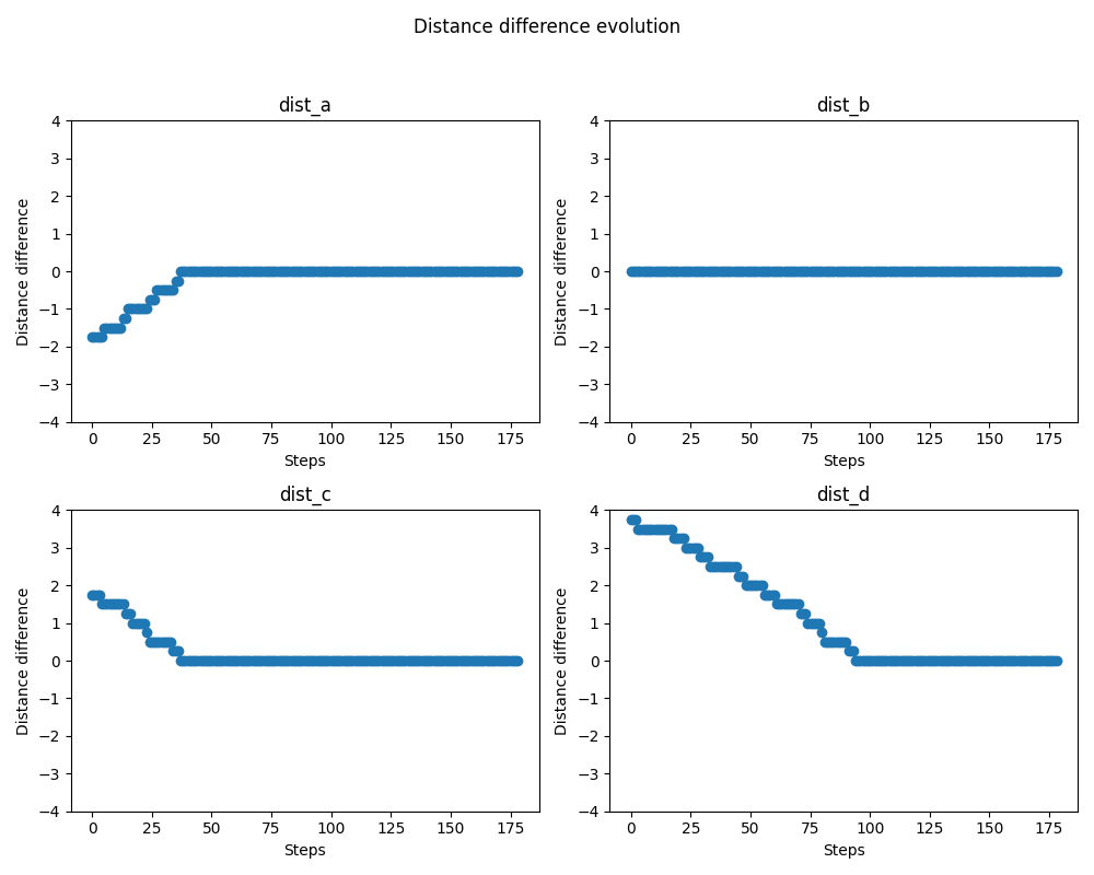
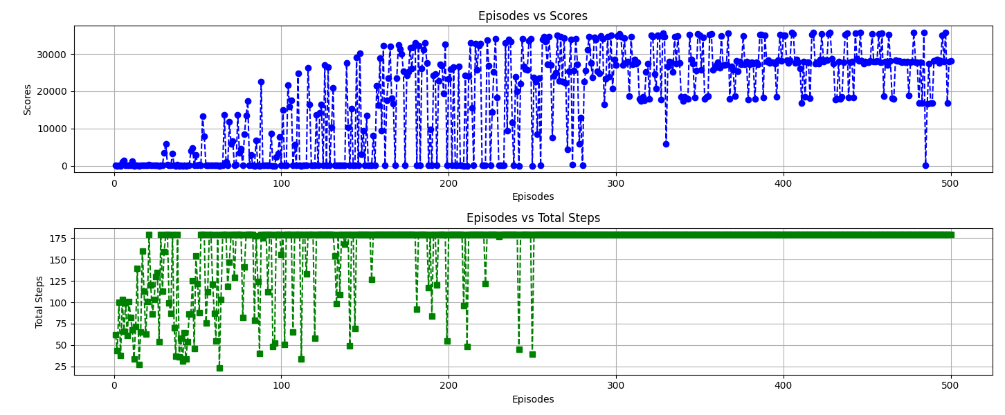
This graph shows how the agent converges to a solution after a number of steps, even from different positions. 
In the video, two phases can be distinguished, the first in which the agent is positioned in a random place and the second in which he lines up between the two cars. example video
Deeper explanation
Rewards
The rewards used were as follows:
1
2
3
4
5
6
7
8
9
10
11
12
13
14
15
16
17
18
19
20
if np.isinf(distance_90) or np.isinf(distance_270):
    return 0

distance_difference = abs(distance_90 - distance_270)

# fixes inifite rewards
if distance_difference < 0.1:
    distance_difference = 0.1

# centered and static
if distance_difference <= 0.17 and abs(speed) < 0.001:
    reward = 200
# penalties if impact
elif distance_difference > 4.5 or abs(speed) > 12:
    reward = -10
# max standar reward = 100 (1/0.01)
else:
    reward = (1/distance_difference)

return reward
They are based on three parts, centred and static, crash forecast and standard reward.
Discretisation
One of the major problems was the discretisation to achieve a finite number of state spaces. The agent must know at all times what is going on in its environment, but if the discretisation is too large, it is possible to lose information that is happening because the state is not updated. This error was detected and solved by getting the best values for the discretisation.
Parameters
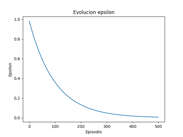
The exploration factor starts at almost 1 and decreases to 0. The decay is exponential and converges at 450 episodes. The learning rate 0.2. And the discount factor at 0.9 to focus on future rewards.
State space
For the state space, we started with the distance difference only, but eventually incorporated the current velocity so that it would be able to remain static without oscillations.

