Armando Mateus – Report June 12, 2026 (Week 34)

Fine‑Tuning or a New Model? Finding the Optimal Dataset Distribution

June 12, 2026

In the previous week, the following guiding questions were raised for this week's work:

Are we fine‑tuning or training a new model?
Why is there a performance degradation when going from 2000 samples to 5000 samples, followed by an improvement at 8000 samples?

To answer these questions, the following workflow was followed:

Analysis of the training script, particularly the section defining the model architecture.
Construction of 16 dataset compositions based on varying the percentages of each maneuver (out of a total of 10 maneuvers).

A. Analysis of the Training Script

The function developed for building the PilotNet model is presented in Code 1. This function is known as "improved PilotNet" and corresponds to an enhancement of NVIDIA's original PilotNet version [1]. The use of this function ensures the creation of a new model initialized with He algorithm weights.

def create_pilotnet_model(input_shape=(120, 160, 3), dropout_rate=0.3):
    model = models.Sequential([
        layers.Input(shape=input_shape),
        
        # Bloque 1
        layers.Conv2D(24, (5, 5), strides=2, padding='valid', kernel_initializer='he_normal'),
        layers.BatchNormalization(),
        layers.Activation('relu'),
        layers.Dropout(dropout_rate * 0.3),
        
        # Bloque 2
        layers.Conv2D(36, (5, 5), strides=2, padding='valid', kernel_initializer='he_normal'),
        layers.BatchNormalization(),
        layers.Activation('relu'),
        layers.Dropout(dropout_rate * 0.3),
        
        # Bloque 3
        layers.Conv2D(48, (5, 5), strides=2, padding='valid', kernel_initializer='he_normal'),
        layers.BatchNormalization(),
        layers.Activation('relu'),
        layers.Dropout(dropout_rate * 0.3),
        
        # Bloque 4
        layers.Conv2D(64, (3, 3), padding='valid', kernel_initializer='he_normal'),
        layers.BatchNormalization(),
        layers.Activation('relu'),
        
        # Bloque 5
        layers.Conv2D(64, (3, 3), padding='valid', kernel_initializer='he_normal'),
        layers.BatchNormalization(),
        layers.Activation('relu'),
        
        # Capas densas
        layers.Flatten(),
        layers.Dense(100, kernel_initializer='he_normal'),
        layers.BatchNormalization(),
        layers.Activation('relu'),
        layers.Dropout(dropout_rate),
        
        layers.Dense(50, kernel_initializer='he_normal'),
        layers.BatchNormalization(),
        layers.Activation('relu'),
        layers.Dropout(dropout_rate * 0.5),
        
        layers.Dense(10, kernel_initializer='he_normal'),
        layers.BatchNormalization(),
        layers.Activation('relu'),
        
        # Salida
        layers.Dense(1, activation='tanh')
    ])
    return model

🔍 Note: The script implements an "improved PilotNet" with He normal initialisation. No pre‑trained weights are loaded. Each training run creates a new model initialised from scratch. This means we are not fine‑tuning; we are training new models each time.

B. Diversity of Dataset Compositions

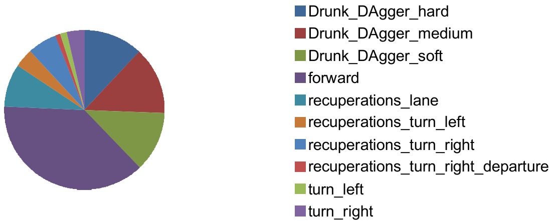
In Town 01 (30 Hz at 10 km/h), samples were taken from the following maneuvers:

Drunk_DAgger_hard: drunk driver with 1 second duration and steering 0.6 (18,334 images)
Drunk_DAgger_medium: drunk driver with 1 second duration and steering 0.45 (21,160 images)
Drunk_DAgger_soft: drunk driver with 1 second duration and steering 0.3 (18,824 images)
Forward: straight driving with ideal steering value 0 (58,123 images)
recuperations_lane: right lane recovery examples from the left lane (13,313 images)
recuperations_turn_left: right lane recovery examples after left turn (5,886 images)
recuperations_turn_right: right lane recovery examples after right turn (9,068 images)
recuperations_turn_right_departure: right lane recovery examples after ending in left lane when turning right (1,547 images)
turn_left: left turn examples (2,100 images)
turn_right: right turn examples (5,420 images)

Figure 1: Original size in number of samples per maneuver obtained in Town01 of Carla at 30Hz at 10Km/h

Figure 1 – Original number of samples per maneuver obtained in Town01 of Carla at 30Hz at 10Km/h; the total number of samples is 153,966.

⚠️ Important limitation: Despite reducing vehicle speed and increasing the sampling rate (more examples per second), the total number of left turn examples was only 7,986 (approximately 5.2% of the total 153,966). This imposes a limit on dataset composition. For example, if 25% of the dataset must correspond to left turn examples (as in Week 33), the maximum possible dataset size would be 31,944 examples.

Table 1. Dataset compositions proposed (percentages per maneuver):

Maneuver / Composition	0	1	2	3	4	5	6	7	8	9	10	11	12	13	14	15
Drunk_DAgger_hard	10	9	8	6	6	5	7	5	20	0	0	0	3	3	5	5
Drunk_DAgger_medium	10	9	8	6	6	5	7	5	0	20	0	0	3	3	5	5
Drunk_DAgger_soft	10	9	8	6	6	5	7	5	0	0	20	0	3	3	5	5
forward	10	19	28	28	28	26	30	30	30	30	30	30	30	30	30	15
recuperations_lane	10	9	8	6	6	10	9	5	0	0	0	20	3	3	5	5
recuperations_turn_left	10	9	8	6	6	10	8	10	10	10	10	10	3	3	5	5
recuperations_turn_right	10	9	8	6	6	10	8	10	10	10	10	10	3	3	5	5
recuperations_turn_right_departure	10	9	8	6	6	10	8	10	10	10	10	10	2	2	5	5
turn_left	10	9	8	15	10	10	8	10	10	10	10	10	20	25	15	20
turn_right	10	9	8	15	20	10	8	10	10	10	10	10	30	25	20	30
Total percentage	100	100	100	100	100	101	100	100	100	100	100	100	100	100	100	100

Table 1 shows the 16 proposed dataset compositions. This contrasts with Week 33's distribution, which only used 3 categories: forward driving (30%), turns (50%), and Drunk-Dagger + recoveries.

C. Video Results – Composition #10

The following videos show autonomous driving performance for Composition #10 at different dataset sizes:

Composition 10 – 2000 samples (baseline)
Video 1
Video 2

Composition 10 – 2000 samples (extra)
Video 3
Video 4

Composition 10 – 10000 samples
Video 5
Video 6

Composition 10 – 15000 samples
Video 7
Video 8

D. Conclusions

About dataset composition:

Autonomous driving experiments in both Town 01 (baseline performance) and Town 02 (generalisation) consistently show better performance for the dataset sizes tested.
Composition #10 demonstrates that including Drunk_DAgger_hard and Drunk_DAgger_medium in driving samples negatively affects autonomous driving performance.
The fact that Composition #3 performs much better than Composition #4 indicates that a balance between the number of left and right turn samples is preferable.

About dataset size:

Increasing dataset size has a direct implication for autonomous driving performance, being especially relevant for generalisation as evidenced in Town 02 driving.
Taking Composition #10 as a reference (where 10% of images correspond to left turns), with the current recording parameters, the maximum viable dataset size is 21,000 samples (given only 2,100 raw left turn samples).
The performance dip at 5k and recovery at 8k observed in some compositions is caused by left-right imbalance due to the scarcity of left turn raw samples. Balanced compositions (like #10) avoid this dip entirely.

E. Next Week Plan (Week 35)

🚀 Proposed work for Week 35:

Expand dataset size by integrating samples from Town 04 – collect samples from Town 01 and Town 04, test on Town 02 and Town 06.
Plan to increase diversity with different weather conditions (rainy and cloudy scenarios).
Make variations on Composition #10 to seek further performance improvements.
Public release – after Week 35 validation, all code, trained models, and dataset compositions will be made available.

F. References

[1] Bojarski, M., et al. (2016): End to end learning for self‑driving cars (PilotNet). arXiv:1604.07316
[2] Mateus, A. (2026): Week 33 report – Dataset balancing & generalisation.
[3] NVIDIA PilotNet Architecture Documentation – Original implementation reference.

— Armando Mateus, Robotics Lab URJC

📌 WEEK 34 SUMMARY – JUNE 12, 2026

🔍 Fine‑tuning or new model? The script trains a new PilotNet from scratch (He initialisation). No fine‑tuning is performed.

📊 16 dataset compositions were built by varying percentages of 10 maneuvers. Composition #10 (10% left, 10% right, 30% forward, 30% recoveries) performed best.

⚠️ 5k dip and 8k recovery explained: Caused by left‑right imbalance due to scarcity of left turn samples (only 2,100 raw). Balanced compositions avoid the dip.

✅ Best model: Composition #10 with 15,000 samples.

🔜 Week 35: Expand with Town 04 samples, add weather diversity, test on Town 02 and Town 06.