Autonomous driving: qlearning algorithm

QLearning

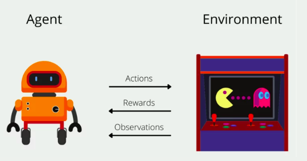
The objective of this project is to develop autonomous driving around a circuit using different machine learning techniques. The main one was QLearning: an algorithm that consists on identifying possible states, perform actions on those states and identify the result of those actions in order to know if the agent did well or not. By repeating this process, known as training, we can obtain an agent that performs relatively well on unknown situations if it has a well determined set of states and actions that result on good behaviour on those states.

Algorithm workflow.

As we have described, the algorithm is based in certain states and actions that when applied, can or cannot help the agent on changing states. In our problem, those actions and states can be defined as:

Actions

The method has five possible actions:

• Going straight
• Turn left and deccelerate
• Turn right and deccelerate
• Sharply turn left and almost stop
• Sharply turn right and almost stop

With this five actions defined, we have a discretized way of driving a car. The actions should be more than enough to tackle through any circuit. If the track is too narrow or its turns are too sharp, the big turning actions will handle it perfectly. If the turns are not that sharp, they can be handled by the smaller turning methods, and if there is any tricky situation, any combination of boths will handle it accordingly.

States

In terms of states, we always have the target to be on the road, whether it is to always try to follow the center, to try to go as fast as possible, to try to follow a “racing line” or whatever the purpose of the training is. As in every possible scenario the car will always have to be on the road, the next states have been defined:

• Centered state: The robot is on top or nearly on top of the center of the track.
• Slightly left state: The robot is situated on the left hand side of the center of the track, like if it followed the left lane.

• Slightly right state: The robot is situated on the right hand side of the center of the track, like if it followed the right lane.

• Sharply left state: The robot is situated on the left hand side of the track, on the verge of exiting the track. At some points of the track, when the robot is on this state it can have a wheel off the track.

• Sharply right state: The robot is situated on the right hand side of the track, on the verge of exiting the track. As with the right one, there are spots where a wheel can touch the grass.

It is important to say that being on these last two states does not actually mean that the robot is almost out of the track: it means that it is almost about to lose perception of the line. The robot can also find himself in this situation if there is a right-hand-side corner coming and it turns left: it will easily lose the visibility of the line even though it is on the track.

This is a visual representation of the QLearning states of the robot:

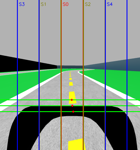
As we can see, the robot will be on state 0 since all the detection points that represent the center of the lane are on the S0 range. Whatever box the red dots are on, that will be the state the robot is currently on.

Reward function

When an action is performed on a certain state, we need to have a way to know which was the result of that action, if it was good for the execution or if it was bad. Let’s say for example that we want to follow the center of the line. If we are on a straight line and we sharply turn right, we wont be following the center of the line anymore, so that is not a good action.

To qualify actions as good or bad, we use reward functions. The reward function analyzes the action taken and its result on the future. An example of reward function would be a function that receives the distance of the center detection to the center of the line and returns a value inversely proportional to the difference: If there is little error, a big reward is given. If the error is too big, a bad reward is given. This reward function would work if we want to train a QLearning agent that follows the center of the road.

QChart

The Q Chart is the way to store all of this information when training an agent. The Qchart is updated every iteration and is is composed of N rows and M columns, with N being the number of states and M being the number of actions. The purpose of the QChart is to tell the agent which action is the best for each state. As said, it is filled progresively with the iterations. In every iteration, the Qchart value for a certain state and an action taken on that state follows the following formula:

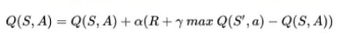
R is the value of the reward function, whilst α and γ are two parameters that we will discuss later and affect the precision of the training.

Training

Now we are going to discuss the training process that can be followed to obtain an agent who can follow the center of the road.

Setup

The training setup will be the same track used for the teleoperator development and for the follow line approach. This track has a lot of left handed turns and just one right handed turn. We will see how that affects the training process and the changes needed to fix it.

The car will be the same deepracer model that we have been using along the project. It will use the control module of V and W and the detection algorithm explained on the previous post.

Execution loop

The training occurs in a continous loop until it has finished. There is an iteration on the loop every time the detection analyzes an image. The workflow is the following:

• Pause the simulation to ensure the robot does not move when computing is done
• Obtain the center of the image in the iteration.
• Use the center obtained as a result of the previously taken action and analyze its result, obtaining the reward function and updating the QChart.
• Unpause the simulation
• Take a new action.

The action will be executed in the time an image the detector receives an image again.

Action decision

When we are training, a criteria must be followed to know which action to take in each moment. This is a very important step on QLearning. As we said above, the QChart stores the best possible actions for each state, but there are two issues with always following the QChart to perform actions:

• The QChart is not initially filled with anything. The algorithm learns on its own and fills the chart with experience, so at the beggining, no actions are better than others.

• Taking always the best possible decision may look like the best way of performing, but it can also mean that the robot is stuck at being “simply decent”. If the robot believes that going slow and on the middle of the track is the best thing, it may lose out on the possibility to learn how to go fast and in the middle of the track, or how to be even more precise.

This two issues can be fixed by adding a percentage of actions taken as random. This means that when an action is going to be taken, there is no guarantee that it will be the best action for that moment. This helps the agent to

• Fill the chart at the beggining of the training
• Discover better (or worse) ways of learning.

This random action decision needs to be regulated: A lot of random actions should be taken on the beggining of the training to fill as much data on the QChart as possible, but a few should be taking on late stages of the training, since too many random actions can ruin the learnt data from the performed training. In order to determinate if we should take a random action or not, we use something called decay factor, who decreases with episodes.

Episodes

Episodes are a way to “reset” the Qlearning training, but they do not delete anything learnt. An episode is a way of telling the agent that there has been a drastical change. Episodes are composed of a number of iterations and they normally change when something very bad happens, for example, exiting the road.

When an episode changes, we are in a good moment to change the decay factor. The decay factor is a number between 0-1 that is compared against a random number. If the random number is smaller than the decay factor, we will take a random action. If not, we will take one from the QChart.

The decay factor does not change with every episode, as they can be too short. It is normally modified at a rate of N episodes. The bigger the episode count to decrement the decay factor, the more random actions the robot will try to explore its environment, but the slower the training will be.

QLearning Training on this project.

Now that the concepts are clear, we will talk through on how QLearning is implemented on this project.

Goal: Following the center of the road.

The main goal of this first QLearning training is to have the car following the center of the road, without going out. For that, we have defined the following parameters.

Reward functions:

The reward function is not static for all the training: It depends on the state. This is done because being on the center state is better than being on the right one, and the pixel difference between states can be 1 or 2, so a linear reward function would give almost the same reward to being on the edge of S0 than to being on the start of S1. The functions are the following:

• When in centered state, the robot will have the highest reward, 100, if it is over the line. If the distance between the center of the detection and the center of the image increases, the reward will reduce gradually until 50 at the edges of the states.

• When in any of the two “safe” side-of-the-center states, the reward will be 30 when we are very close to being back into the center state and close to 15 when we are almost entering the dangerous states.

• When we are on the verge of leaving on any of the two sides, the reward will be 10 when we are almost joining the left-right states back or 0 when we are almost crashing.

If the robot crashes, it will always get a reward of -100. This is done to tell the agent that crashing is the worst possible scenario and that it should always try to be avoided.

Alpha and Gamma

As we said before, there are two parameters present when updating the QChart: α and γ.

α

Alpha represents the total weight of the new observation into the QChart, the learning rate. A lower alpha value would mean that the previously stored action will be more important than the newly observed. This will lead to slower but more precise trainings. If alpha is high, it will mean the opposite: Training will be faster as the taken action will be more important, but it can lead to convergence problems if the training is not well adjusted.

For our training, we have used an alpha of 0.5, obtaining a good balance between convergence and a not-too-big training time.

γ

In the QLearning formula, we see that we take into account the higest QChart value stored for the state we have ended on after taking the action. Gamma represents the discount factor for that value. Applying a big gamma means that the future action, or the action that should be taken when the decision takes place, will be very important. A lower gamma factor will mean that the best action of the future state is not considered important. This could mean to the agent taking actions that are not optimal since it can doubt between which action to take.

In our simulation, gamma is 0.7. This gives a good weight to the future action helping the robot in closed turns.

It can also be interesting to have a dynamically growing gamma, since at the beggining of the training the chart is not fully filled and you cannot assume that the highest reward for an state on an early stage of the training will be 100% the best action to take, whilst in the future you should be able to assume that with a converging training.

Episode resetting

We have mentioned episodes as key parts of the Qlearning training process. Resetting the episodes gives an oportunity to change the environment to facilitate training.

In this training, whenever an episode is finished, the robot places himself on a random different position. The list of positions is not entirely random but in the list, every position is picked randomly. This are the positions and the orientation of the robot on each:

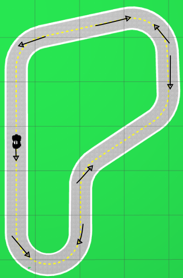
The direction of the line shows where the car faces when spawned.

As it is seen, there are arrows that point on clockwise sense of the track and another ones on counterclockwise. This is done since the track only has a single right hand corner, training always on the same direction of the track would result on the car not learning how to take right handed corners. By balancing the amount of right and left corners, we can obtain a behaviour that also could be ported to a different circuit with more right hand side turns.